This paper is available on arxiv under CC 4.0 license.
Authors:
(1) Kiriaki Frangias;
(2) Andrew Lin;
(3) Ellen Vitercik;
(4) Manolis Zampetakis.
Table of Links
Warm-up: Agents with known equal disutility
Agents with unknown disutilites
Conclusions and future directions, References
B Omitted proofs from Section 2
C Omitted proofs from Section 3
D Additional Information about Experiments
4 Experiments
In the following section, we present experiments that test our models and algorithm. We evaluate the impact of our algorithm on the principal’s utility compared to when she chooses not to incentivize agents, the efficacy of our algorithm in returning correct pairwise comparisons, and the robustness of our model to noisy values of ψ and π.
Experimental procedure. Unless otherwise specified, we keep the following set of hyperparameter values across our experiments: π = 0.8, δ = 0.01, s = 100, n = 100, ψ¯ = 2, and ψ = 0.01. Peer grading is an example of a setting where s = n since the number of assignments is the same as the number of students. In Appendix D, we include experiments with a broad variety of parameter settings.
Since we add noise to our model in these experiments, CrowdSort may not catch all bad agents and thus may return conflicting comparisons. We discard all conflicting comparisons (see Algorithm 4 in Appendix D). Despite this pessimistic post-processing strategy, our experiments show that we can recover most comparisons even under noise.
4.1 Principal’s utility


The empirical utilities are calculated as follows. Let m be the number of agents not identified as “bad” by CrowdSort and k be the number of comparisons after post-processing. We set λ = 2 to be the principal’s per-comparison utility and define

to be her empirical utility for running CrowdSort with p∗, v∗ , and r∗ defined in Equations (1) and (2). Similarly

is her expected utility for performing all comparisons herself, where 2n log n is the expected number of comparisons required by quicksort (this value could easily be adjusted for any sorting algorithm). For ease of comparison, the y-axis is scaled by dividing all values by the baseline utility U0.
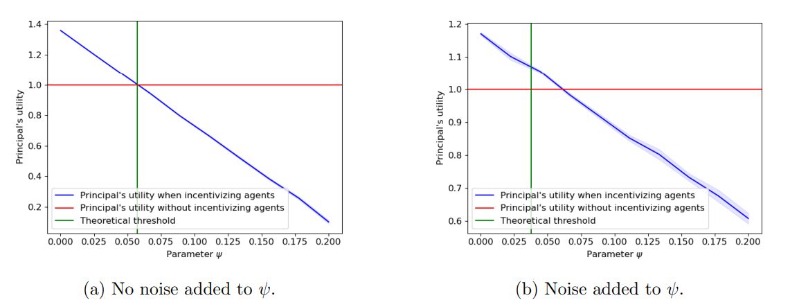
We note that the size of the confidence interval decreases with π. For small values of π, a small number of agents are “good”, even though all agents exert effort. Then with higher probability, k will be small. This corresponds to higher variance in the principal’s utility across trials.
In Figure 1b, we add noise to the parameter ψ and analyze the effect on the principal’s utility. We sample the disutility of each agent independently and identically from the distribution Uniform(ψ − 0.5ψ, ψ + 0.5ψ). However, we still calculate p∗, v∗, and r∗ from Equations (1) and (2) using ψ itself instead of the noisy version. The blue shading corresponds to a 90% confidence interval across 50 trials.
Discussion. Comparing Figures 1a and 1b, we can see that even when noise is added to our model, our theoretical threshold is close to the point at which the principal’s utility from running CrowdSort dips below their utility from performing all comparisons herself. This demonstrates that our theoretical results are robust to noise in the model.
When adding noise to ψ, the principal must pay fewer agents because fewer are incentivized to exert effort. Thus, we see a steeper decline in Figure 1a compared to 1b.

4.2 Number of pairwise comparisons returned

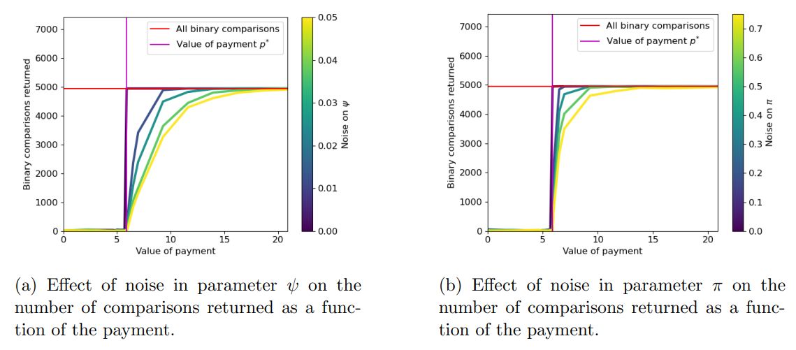
Discussion. These experiments show that our algorithm retrieves all comparisons in the absence of noise. Moreover, even when a large amount of noise is added to ψ or π, our algorithm returns almost all of the comparisons with sufficient payment, despite the postprocessing phase excluding any conflicting comparison, again illustrating our algorithm’s robustness.

4.3 Optimization problem

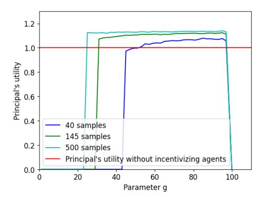
Discussion. For suitable values of g, approximately 40 samples are required for the utility of the principal under our model to surpass the utility she would get, if she were to perform all pairwise comparisons herself. We also notice that the principal’s utility increases as we increase either g or the number of samples. This result is shown in the multi-colored plots in Figure 3. Therefore, even for a small number of samples, the principal’s utility when implementing CrowdSort is well above her utility if she performed all comparisons on her own.
This paper is available on Arxiv under CC 4.0 license.

