Authors:
(1) Davide Viviano, Department of Economics, Harvard University;
(2) Lihua Lei, Graduate School of Business, Stanford University;
(3) Guido Imbens, Graduate School of Business and Department of Economics, Stanford University;
(4) Brian Karrer, FAIR, Meta;
(5) Okke Schrijvers, Meta Central Applied Science;
(6) Liang Shi, Meta Central Applied Science.
Table of Links
Empirical illustration and numerical studies
2 Setup

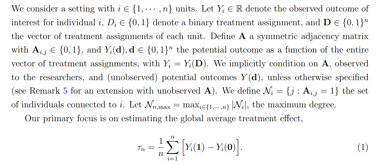
The overall effect defines the effect if all units had received the treatment compared to none of the individuals receiving the treatment. Table 1 summarizes the notation.
2.1 Spillover effects
Next, we impose restrictions on the spillover effects.
Assumption 1 (First-order local interference). For i ∈ {1, · · · , n},

Assumption 1 states that spillovers occur between neighbors and allows for arbitrary dependence of potential outcomes with neighbors’ assignments. One-degree neighborhood dependence follows similarly to Leung [2020], Li and Wager [2022], and it is consistent with models often used in applications, e.g., Cai et al. [2015], Sinclair et al. [2012], Muralidharan and Niehaus [2017]. Athey et al. [2018] provide a framework for testing Assumption 1. The reader may refer to Remark 2 for higher-order interference. Higher-order interference can be accomodated, although, in practice, higher order effects can be small and difficult to detect.
We will refer to τn,µ as the overall effect in Equation (1) to make the dependence of τn on (µ1, · · · , µn) explicit. We do not assume that we know or can estimate consistently µi . (Because the functions µi and their classes M0,i,M1,i are indexed by i, such functions cannot be consistently estimated.) Instead, we allow for arbitrary classes M1,i,M0,i of potential outcome functions, as long as such classes satisfy the conditions below. These classes have to be both sufficiently large in order to accomodate rich structures in the data, as well as satisfy some restrictions to be able to estimate features of causal effects.
Assumption 2 (Sufficiently large function class). For all i ∈ {1, · · · , n}, d ∈ {0, 1},

Assumption 2 directly holds if Md,i contains all functions, and, requires that the function class under consideration is sufficiently large otherwise. Specifically, (i) the function class Md,i contains each function and its opposite. This restriction does not impose restrictions on exposure mappings and allows for arbitrary sign flips.[4] Condition (ii) states that there exists one function in the admissible function class that is constant and positive. Condition (ii) is a regularity condition that guarantees non-degenerate solutions in worst-case scenarios studied in the following section. Condition (iii) considers a product space of potential outcome functions. These conditions are not restrictive, and they hold if M0,i,M1,i can contain arbitrary functions. Below we impose the main restrictions on the function class.
Assumption 3 (Restricted class of potential outcome models). For all i ∈ {1, · · · , n}, d ∈ {0, 1}

Assumption 3 imposes two restrictions. Condition (i) states that potential outcomes are uniformly bounded.[5] Condition (ii) is our main restriction on the exposure mapping. Condition (ii) is attained if M1,i,M0,i are Lipschitz function classes in the share of treated neighbors. Condition (ii) states that potential outcomes vary in the share of neighbors’ treatments by at most αiϕ¯ n. Here ϕ¯ n captures the magnitude of (largest) spillovers, and αi captures individual-level heterogeneity.
The component ϕ¯ n depends on n and will play an important role in our asymptotic analysis as n → ∞. We focus on settings where ϕ¯ n is small (i.e., ϕ¯ n = o(1) as n → ∞), in the spirit of a local asymptotic framework [e.g. Hirano and Porter, 2009], but its convergence rate can be arbitrarily slow. These scenarios formalize the idea that spillover effects (and possibly but not necessarily also overall treatment effects τn) are local to zero. For example, in an information campaign, we might expect spillover (and direct) effects to be small but non-negligible for inference, as often occurs in online experiments [Karrer et al., 2021]. We show how different magnitudes of spillover effects justify different designs.

Assumption 4 formalizes the local asymptotic framework considered here: spillovers converge to zero, but the rate can be arbitrary slow up to a term that depends on the squared maximum degree.[6] Assumption 4 holds for arbitrary rates of convergence of the spillover effects ϕ¯ n for networks with bounded degree [e.g. De Paula et al., 2018, where Nn,max is bounded], and requires faster rates of ϕ¯ n (smaller spillover effects), for dense networks. We conclude this discussion with examples and remarks

Remark 1 (Local asymptotics and direct effect). Our local asymptotic framework also allows direct treatment effects (and global effects) to be local to zero. Specifically, it is possible that τn = o(1) at arbitrary rate, e.g., at the same rate as ϕ¯ n. Therefore, our local asymptotic assumption does not require that spillover effects are local to the global effect (since τn can also converge to zero). Instead, our local asymptotics formalizes settings where the noise-to-signal ratio decreases slower than n −1/2 .
Remark 2 (Higher order interference and endogenous peer effects). Our setting generalizes to higher-order interference in two scenarios.
First, suppose that friends up to degree d < ∞ generate spillovers in magnitude similar to first-degree friends. Our results extend after we define the set of friends as the set of friends up to degree d, and ϕ¯ n the largest effect that such friends generate. Sparsity restrictions on the largest degree in Assumption 4 are with respect to the number of friends up to degree d. In the second scenario, suppose that the assumption of first-order effects approximates higher-order effects up to a term of smaller order than first-order effects. Specifically, suppose that Yi(d) = µi(di , dNi )+O(hn), for some hn → 0. Our results hold if hn = o(1/n), capturing the idea that first-order effects ϕ¯ n are larger than second-order effects. In Appendix B we provide an example and sufficient conditions for the approximation error due to higher order interference being of order o(1/n) in the presence of endogenous peer effects [Bramoull´e et al., 2009, Manski, 1993], where the individual outcome depends on other units’ outcomes.
In practice, higher-order effects can be small, leading to under-powered studies, especially when individuals have many friends and first order effects capture most of the spillovers. This motivates our focus on first order effects.
2.2 Experimental design and estimation
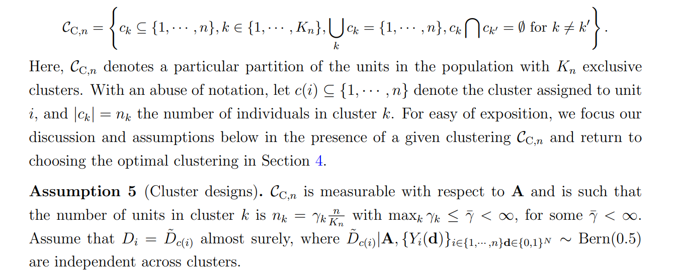
Next, we turn to the class of designs and estimators considered here. Define a clustering of size Kn as a set of sets of indicators satisfying

Assumption 5 states the clustering is constructed using information from the adjacency matrix only (i.e., it is independent of potential outcomes), clusters are proportional in size[7] , and individuals in a given cluster are all assigned either treatment or control with equal probability. Assumption 5 restricts the class of designs to cluster designs, motivated by our focus on overall treatment effects, and empirical practice.[8]
Motivated by standard practice both in industrial applications and in field experiments with clusters [Baird et al., 2018], we consider estimators obtained by simple difference in means between treated and control clusters. Because P(Di = 1) = 1/2, we construct a (biased) estimator of treatment effects as

The estimator ˆτ cl n (CC,n) is a simple difference in means between treated and control units, that normalizes by the probability of treatment. Therefore, ˆτ cl n (CC,n) depends on the clustering CC,n only because the distribution of the treatments depends on the clusters under Assumption 5. Studying the estimator in Equation (3) is a natural starting point for the analysis of cluster experiments. Variants of difference in means estimators (possibly also with regression adjustments discussed in Remark 3) are often used or studied in practice [Holtz et al., 2020, Karrer et al., 2021, S¨avje et al., 2021]. One could also normalize each sum in Equation (3) by the number of treated and control units (instead of using knowledge about the treatment probability). This would improve the stability of the estimators, but complicate the analysis of the estimators’ properties when the number of treated units is stochastic (e.g., when clusters have different size).[9]
Remark 3 (Covariate adjustment). Our framework directly generalizes to settings that use covariate adjustment for baseline outcomes. Denote ¯µi an arbitrary predictor for µi(0) that only uses information from some arbitrary baseline observable characteristics (i.e., does not depend on the treatments or end-line outcomes in the experiment). The estimator with such an adjustment takes the form

Our analysis continues to hold after defining the outcome of interest Yi − µ¯i .
Remark 4 (Alternative estimators). Alternative estimators studied in the literature are inverse probability weights estimators [e.g., Aronow and Samii, 2017, Ugander et al., 2013]. Unless researchers impose additional restrictions on the exposure mapping, in the network context, these estimators can be subject to instability of the propensity score because they reweight by the inverse probability that all friends of a given individual are either under treatment or control. A different alternative are model-based estimators, which however can be subject to model misspecification.

[4] Our results also hold if instead of imposing (i) we assume that the difference between µi(1, d) − µi(1), µi(0, d) − µ(0) can be symmetric for all d ∈ {0, 1} n.
[5] This restriction is common in the literature, e.g., Kitagawa and Wang [2021], and can be relaxed by assuming random sub-gaussian potential outcomes.
[6] The restriction on the maximum degree squared can be sharpened by imposing restrictions on the average second-order degree, omitted for expositional convenience.
[7] This restriction is sufficient but not necessary for our analysis, and it is imposed for expositional convenience, as the rates of convergence only depend on n and Kn (population size and number of clusters) instead of also the dimension of the largest and smallest cluster. It is possible to relax such an assumption by assuming that PKn k=1 γ 2 k /Kn = O(1).
[8] Saturation designs [e.g. Baird et al., 2018] would also be interesting to study if researchers are interested in estimands other than the overall treatment effect, such as the effect of treating a certain percentage of individuals in a given cluster. We leave saturation designs to future research.
[9] With a stochastic number of treated units, the estimators with and without normalization are equivalent up-to an error of order O(1/ √ Kn).
This paper is available on arxiv under CC 1.0 license.

