Authors:
(1) Davide Viviano, Department of Economics, Harvard University;
(2) Lihua Lei, Graduate School of Business, Stanford University;
(3) Guido Imbens, Graduate School of Business and Department of Economics, Stanford University;
(4) Brian Karrer, FAIR, Meta;
(5) Okke Schrijvers, Meta Central Applied Science;
(6) Liang Shi, Meta Central Applied Science.
Table of Links
Empirical illustration and numerical studies
4 Choosing the cluster design
In this section, we turn to the question of designing the optimal clustering. The following theorem characterizes the objective function.

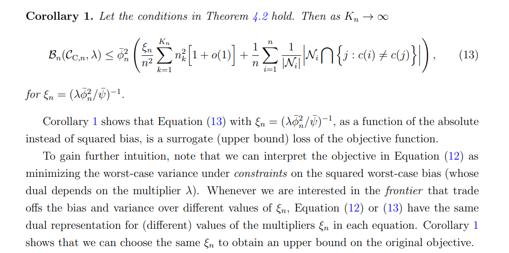
Theorem 4.1 characterizes the objective function as a function of the covariance between units in the same cluster, bounded by ψ¯, the between-clusters variation (average of n 2 k ), the size of the spillover effects ϕ¯ n and the “cluster impurity”, i.e., the average number of friends of a given individual assigned to a different cluster. The constant λ defines the relative importance weight of the bias compared to the variance.
After simple re-arrangement, and assuming that the worst-case spillover effects are homogenous across units (αi = 1 for all i) [11], Theorem 4.1 provides a simple-to-compute metric for ranking (a few) given clusters

4.1 Causal clustering: objective and algorithm
The task of estimating the best clustering over a large class is challenging because the number of connections between different clusters enters non-linearly in Equation (12). As a first step, we rewrite the objective function as a function of the absolute (instead of squared) bias.
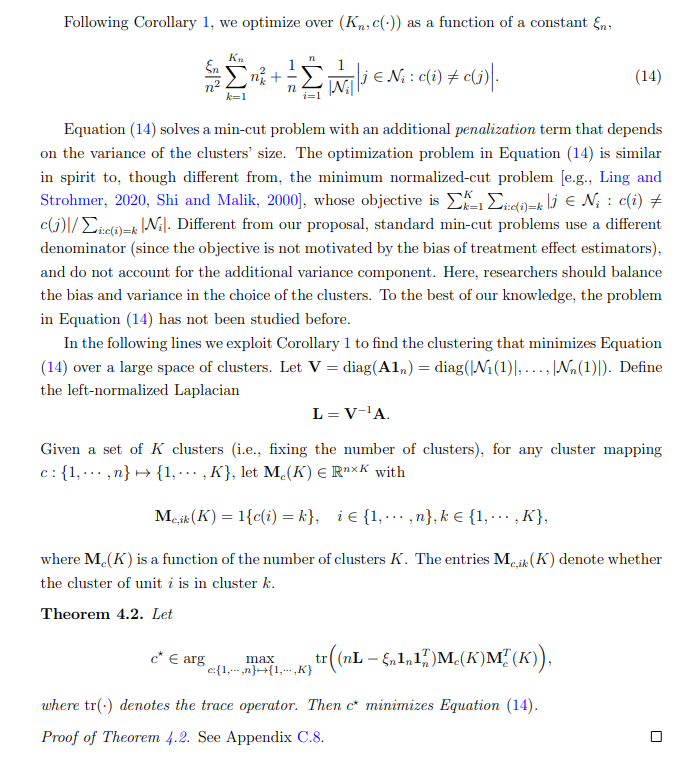
Theorem 4.2 formalizes the optimization problem as a trace-optimization program, for fixed number of clusters K. Theorem 4.2 does not characterize a convex optimization program, but it provides a natural starting point to study convex relaxations of the proposed optimization problem. To obtain a convex relaxation, we relax the constraint on the matrix X(K) = Mc(K)MT c (K). We propose solving the following semi-definite programming (SDP) problem (for given number of clusters K):

where Equation (15) defines a sequence of semi-definite optimization programs, each indexed by the number of clusters K. The main distinction between Equation (14), and Equation (15) is that the matrix X(K) must be positive-definite, but does not necessarily contains binary entries only. Let Xˆ (K) be the solution of (15), for given K, that can be obtained using off-the-shelf optimization routines. We then apply the K-means algorithm [Bradley et al., 2000] on the first K eigenvectors of Xˆ (K) to retrieve the mapping c. [12] Finally, we compare solutions for different values of K and choose the clustering with the largest objective. Equation (15) is a convex relaxation of the problem in Theorem 4.2 because it substitutes the original constraint on X to contain binary entries with a semi-definite constraint, and then retrives the clusters via K-means clustering on the matrix X(K) directly. Such convex relaxations are common in the clustering literature and have been widely studied both from theoretical and numerical perspective, see Hong et al. [2021] for a review.
In summary, the complete algorithm (Algorithm 1) solves a sequence of semi-definite trace-optimization problems, each indexed by a different value of K, and report the clustering (and corresponding number of clusters) that leads to the largest objective.
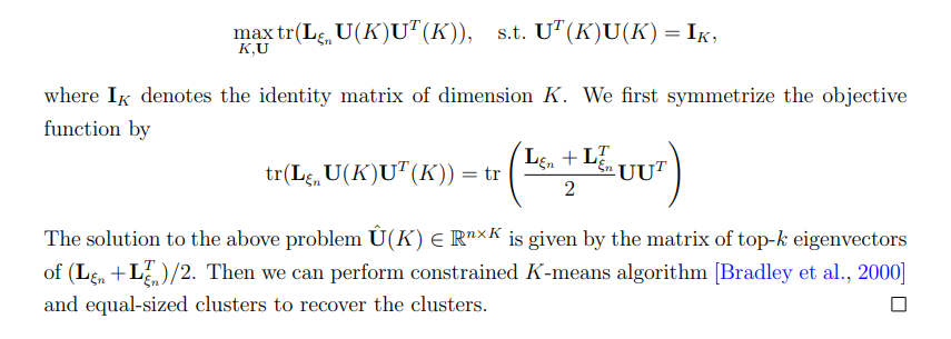
Remark 6 (Spectral relaxation). Unlike the minimum normalized cut, there is no simple spectral relaxation of the optimization problem in Theorem 4.2, unless all clusters are equally sized. For the special case where all clusters are equal-sized, (15) can be relaxed to
Algorithm 1 Causal Clustering
Require: Adjacency matrix A, K, K¯ smallest and largest number of clusters, ξn. 1: for K ∈ {K, · · · , K¯ } do a: Solve Equation (15) and obtain Xˆ (K) as the minimized of Equation (15) b: Retrive the clusters cK via K-means algorithm on the first K eigenvectors of Xˆ (K) c: Compute the objective function corresponding to the chosen clustering in (14) 2: end for 3: return Clustering with the lowest objective function in (14).
4.2 Worst-case mean squared error
We conclude this section by extending our results (Theorem 4.2) to show (i) how to allow for heterogeneity in covariances between individuals and (ii) that the worst-case mean-squared error coincides with the sum of the worst-case bias and variance.
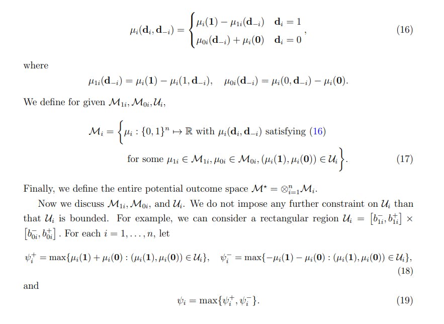
Before doing so, we need to introduce some additional notation. Without loss of generality, for unit i, we decompose the potential outcome function µi(di , d−i) into four components
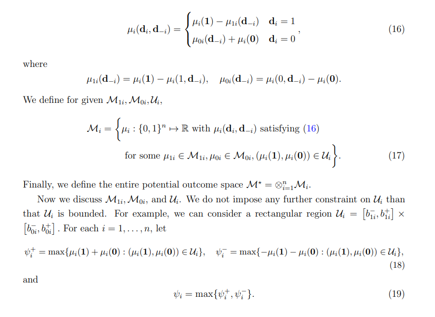
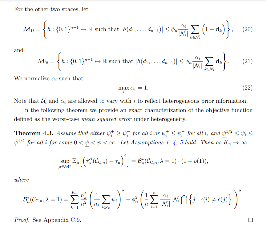
The following corollary shows when the worst-case mean-squared error and the sum of the worst-case bias and variance coincide and when (11) holds with equality. The latter is important because it justifies the objective function (12) as an ex-ante assessment of the worst-case mean square error for a given clustering.


[11] All our results extend to different choices of αi , although we think that αi = 1 is a natural choice in practice, which mimics applications where individuals are assumed to depend on the share of treated friends.
[12] K-means on the K largest eigenvectors of Xˆ (K) is a well-studied problem in the literature on spectral clustering algorithms [Von Luxburg, 2007].
This paper is available on arxiv under CC 1.0 license.

