
Table Of Links
2 FLATTENING AND ARC APPROXIMATION OF CURVES
3 EULER SPIRALS AND THEIR PARALLEL CURVES
5 ERROR METRICS FOR APPROXIMATION BY ARCS
7 CONVERSION FROM CUBIC BÉZIERS TO EULER SPIRALS
CONCLUSIONS, FUTURE WORK AND REFERENCES
RESULTS
We present two versions of our stroking method: a sequential CPU stroker and the GPU compute shader outlined in Section 8. Both versions can generate stroked outlines with line and arc primitives. We focused our evaluation on the number of output primitives and execution time, using the timings dataset provided by Nehab [2020], in addition to our own curve-intensive scenes to stress the GPU implementation. We present our findings in the remainder of this section.
9.1 CPU: Primitive Count and Timing
We measured the timing of our CPU implementation, generating both line and arc primitives, against the Nehab and Skia strokers, which both output a mix of straight lines and quadratic Bézier primitives. The results are shown in Figure 15. The time shown is the total for test files from the timings dataset of Nehab [2020], and the tolerance was 0.25 when adjustable as a parameter. Similarly to Nehab [2020]’s observations, Skia is the fastest stroke expansion algorithm we measured.
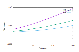
The speed is attained with some compromises, in particular an imprecise error estimation that can sometimes generate outlines exceeding the given tolerance. We confirmed that this behavior is still present. The Nehab paper proposes a more careful error metric, but a significant fraction of the total computation time is dedicated to evaluating it. We also compared the number of primitives generated, for varying tolerance values from 1.0 to 0.001.
The number of arcs generated is significantly less than the number of line primitives. The number of arcs and quadratic Bézier primitives is comparable at practical tolerances, but the count of quadratic Béziers becomes more favorable at finer tolerances. The vertical axis shows the sum of output segment counts for test files from the timings dataset, plus mmark70k (as described in more detail in Section 9.2), and omitting the waves example1 .
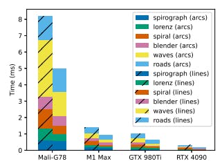
9.2 GPU: Execution Time
We evaluated the runtime performance of our compute shader on 4 GPU models and multiple form factors: Google Pixel 6 equipped with the Arm Mali-G78 MP20 mobile GPU, the Apple M1 Max integrated laptop GPU, and two discrete desktop GPUs: the mid-2015 NVIDIA GeForce GTX 980Ti and the late-2022 NVIDIA GeForce RTX 4090. We authored our entire GPU pipeline in the WebGPU Shading Language (WGSL) and used the wgpu [6] framework to interoperate with the native graphics APIs (we tested the M1 Max on macOS via the Metal API; the mobile and desktop GPUs were tested via the Vulkan API on Android and Ubuntu systems).
We instrumented our pipeline to obtain fine-grained pipeline stage execution times using the GPU timestamp query feature supported by both Metal and Vulkan. This allowed us to collect measurements for the curve flattening and input processing stages in isolation. We ran the compute pipeline on the timings SVG files provided by Nehab [2020]. The largest of these SVGs is waves (see rendering (a) in Figure 20) which contains 42 stroked paths and a total of 13,308 path segments. We authored two additional test scenes in order to stress the GPU with a higher workload.
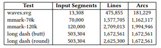
The first is a very large stroked path with ~500,000 individually styled dashed segments which we adapted from Skia’s open-source test corpus. We used two variants of this scene with butt and round cap styles. For the second scene we adapted the Canvas Paths test case from MotionMark [1], which renders a large number of randomly generated stroked line, quadratic, and cubic Bézier paths. We made two versions with different sizes: mmark-70k and mmark-120k with 70,000 and 120,000 path segments, respectively. Table 2 shows the payload sizes of our largest test scenes. The test scenes were rendered to a GPU texture with dimensions 2088x1600.
The contents of each scene were uniformly scaled up (by encoding a transform) to fit the size of the texture, in order to increase the required number of output primitives. As with the CPU timings, we used an error tolerance of 0.25 pixels in all cases. We recorded the execution times across 3,000 GPU submissions for each scene. Figures 17 and 18 show the execution times for the two data sets. The entire Nehab [2020] timings set adds up to less than 1.5 ms on all GPUs except the mobile unit. Our algorithm is ~14× slower on the Mali-G78 compared to the M1 Max but it is still

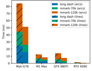
 capable of processing waves in 3.48 ms on average. We observed that the performance of the kernel scales well with increasing GPU ability even at very large workloads, as demonstrated by the orderof-magnitude difference in run time between the mobile, laptop, and high-end desktop form factors we tested. We also confirmed that outputting arcs instead of lines can lead to a 2× decrease in execution time (particularly in scenes with high curve content, like waves and mmark) as predicted by the lower overall primitive count.
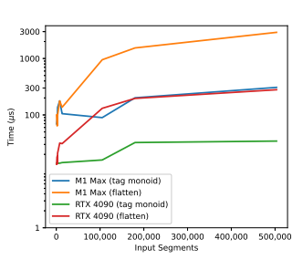
9.3 GPU: Input Processing
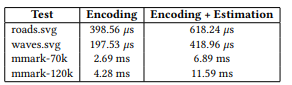
Figure 19 shows the run time of the tag monoid parallel prefix sums with increasing input size. The prefix sums scale better at large input sizes compared to our stroke expansion kernel. This can be attributed to a lack of expensive computations and high controlflow uniformity in the tag monoid kernel. The CPU encoding times (prior to the GPU prefix sums) for some of the large scenes is shown in Table 3. Our implementation applies dashing on the CPU.
It is conceptually straightforward to implement on GPU; the core algorithm is prefix sum applied to segment length, and the Euler spiral representation is particularly well suited. However, we believe the design of an efficient GPU pipeline architecture involves comples tradeoffs which we did not sufficiently explore for this paper. Therefore the dash style applied to the long dash scene was processed on the CPU and dashes were sequentially encoded as individual strokes. Including CPU-side dashing, the time to encode long dash on the Apple M1 Max was approximately 25 ms on average, while the average time to encode the path after dashing was 4.14 ms.
Our GPU implementation targets graphics APIs that do not support dynamic memory allocation in shader code (in contrast to CUDA, which provides the equivalent of malloc). This makes it necessary to allocate the storage buffer in advance with enough memory to store the output, however, the precise memory requirement is unknown prior to running the shader. We augmented our encoding logic to compute a conservative estimate of the required output buffer size based on an upper bound on the number of line primitives per input path segment.
We found that Wang’s formula [7] works well in practice, as it is relatively inexpensive to evaluate, though it results in a higher memory estimate than required (see Table 4). For parallel curves, Wang’s formula does not guarantee an accurate upper bound on the required subdivisions, which we worked around by inflating the estimate for the source segment by a scale factor derived from the linewidth. We observed that enabling estimation increases
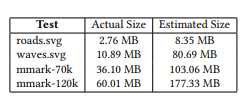
177.33 MB by 2–3× on the largest scenes but overall the impact is negligible when the scene size is modest
Authors:
This paper is