
Table Of Links
2 FLATTENING AND ARC APPROXIMATION OF CURVES
3 EULER SPIRALS AND THEIR PARALLEL CURVES
5 ERROR METRICS FOR APPROXIMATION BY ARCS
7 CONVERSION FROM CUBIC BÉZIERS TO EULER SPIRALS
CONCLUSIONS, FUTURE WORK AND REFERENCES
CONVERSION FROM CUBIC BÉZIERS TO EULER SPIRALS
The Euler spiral segment representation of a curve is useful for computing near-optimal flattened parallel curves, but standard APIs and document formats overwhelmingly prefer cubic Béziers as the path representation. Many techniques for stroke expansion described in the literature apply some lowering of cubic Bézier curves to a simpler curve type that is more tractable for evaluating the parallel curve. Computing parallel curves directly on cubic Bézier curve segments is not very tractable.
In particular, the widely cited Tiller-Hanson algorithm [23] performs well for quadratic Béziers but significantly worse for cubics. A typical pattern for converting from one curve type to another is adaptive subdivision. An approximate curve is found in the parameter space of the target curve family. The error of the approximation is measured. If the error exceeds the specified tolerance, the curve is subdivided (typically at 𝑡 = 0.5), otherwise the approximation is accepted.
Subdivisions are also indicated at special points; for example, since quadratic Béziers cannot represent inflection points, and geometric Hermite interpolation is numerically unstable if the input curve is not convex, lowering to quadratic Béziers also requires calculation of inflection points and subdividing there. A good example of this pattern is Nehab [2020]. One advantage of Euler spirals over quadratic Béziers is that they can represent inflection points just fine, so it is not necessary to solve for the inflection points, or do additional subdivision.
Avoiding these alleviates the need for conditional logic and case analysis, which makes the algorithm more amenable to GPU execution. The approach in this paper is another variant of adaptive subdivision, with two twists. First, it’s not necessary to actually generate the approximate curve to measure the error. Rather, a straightforward closed-form formula accurately predicts it.
The second twist is that, since compute shader languages on GPUs typically don’t support recursion, the stack is represented explicitly and the conceptual recursion is represented as iterative control flow. This is an entirely standard technique, but with a clever encoding the entire state of the stack can be represented in two words, each level of the stack requiring a mere single bit.
7.1 Error prediction
A key step in approximating one curve with another is evaluating the error of the approximation. A common approach (used in Nehab [2020] among others) is to generate the approximate curve, then measure the distance, often by sampling at multiple points on the curve. All this is potentially slow, with the additional risk of underestimating the error due to undersampling. Our approach is different. In short, we perform a straightforward analytical computation to accurately estimate the error.
Our approach to the error metric has two major facets. First, we obtain a secondary cubic Bézier which is a very good fit to the Euler spiral, then we estimate the distance between that and the source cubic. Due to the triangle inequality, the sum of these is a conservative estimate of the true Fréchet distance between the cubic and the Euler spiral. For mathematical convenience, the error estimation is done with the chord normalized to unit distance; the actual error is scaled linearly by the actual chord length.
The cubic Bézier approximating the Euler spiral is one in which the distance of each control point from the endpoint is𝑑 = 2 3(1+cos 𝜃 ) , where 𝜃 is the angle of the endpoint tangent relative to the chord. This is a generalization of the standard approximation of an arc. It
should be noted that this is not in general the closest possible fit, but it is computationally tractable and has near-uniform parametrization. In general it has quintic scaling; if an Euler spiral segment is divided in half, the error of this cubic fit decreases by a factor of 32. A good estimate of this error is:
4.6255 × 10⁻⁶ |𝜃0 + 𝜃1 | 5 + 7.5 × 10⁻³ |𝜃0 + 𝜃1 | 2 |𝜃0 − 𝜃1 |
The distance between two cubic Bézier segments can be further broken down into two terms; in most cases, the difference in area accurately predicts the Fréchet distance between the curves. Two cubic Béziers with the same area and same tangents tend to be relatively close to each other, but there is some error stemming from the difference in parametrization. Area of a cubic Bézier segment is straightforward to compute using Green’s theorem:
𝑎 = 3 20 (2𝑑0 sin𝜃0 + 2𝑑1 sin𝜃1 − 𝑑0𝑑1 sin(𝜃0 + 𝜃1))
The conservative Fréchet distance estimate is 1.55 the absolute difference in area between the source cubic and the Euler spiral approximation. The final term for imbalance is as follows, with ¯𝑑0 and ¯𝑑1 representing the distance from the endpoints of the Euler approximation and 𝑑0 and 𝑑1 the corresponding distance in the source cubic segment, as in the area calculation above:
(0.005|𝜃0 + 𝜃1 | + 0.07|𝜃0 − 𝜃1 |)√︃ ( ¯𝑑0 − 𝑑0) 2 + ( ¯𝑑1 − 𝑑1) 2
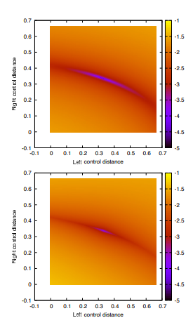
The total estimated error is the sum of these three terms. We have validated this error metric in randomized testing. For values of 𝜃 between 0 and 0.5, and values of 𝑑 between 0 and 0.6, this estimate is always conservative, and it is also tight: over Bézier curves generated randomly with parameters drawn from a uniform distribution in this range, the mean ratio of estimated to true error is 1.656.
A visualization of combined error metric is shown in Figure 10, comparing measured and approximate error for a slice of the parameter space, fixing the endpoint angles to 0.1 and 0.2, and varying the distance from both endpoints to the control point.
7.2 Geometric Hermite interpolation
Given tangent angles relative to the chord, finding the Euler spiral segment that minimizes total curvature variation is a form of geometric Hermite interpolation. There are a number of published solutions to this problem, involving nontrivial numerical solving techniques: gradient descent [13], bisection [24], or Newton iteration [3].
A more direct approach is to approximate the function as a reasonably low-order polynomial in terms of the endpoint angles. Our approach is to use a 7th order polynomial, which is more precise than the 3rd order polynomial proposed in Reif and Weinmann [2021], at only modest increased cost.
The exact coefficients used are presented in Appendix A. 7.3 Cusp handling There are two types of cusps that must be handled in the stroke expansion problem. One is when the input cubic Bézier contains a cusp (or near-cusp, which is prone to numerical robustness issues),
and one is when the parallel curve contains cusps. This section will describe both in order. A Bézier curve is expressed in parametric form, and its derivative with respect to the parameter can be zero or nearly so, causing serious numerical problems for many stroke expansion algorithms. In the limit, as the Bézier curve describes a semi-cubical parabola, the curvature can become infinite. Our approach leverages the conversion to Euler spiral segments, which have finite curvature.
The geometric Hermite interpolation depends on accurate tangents at the endpoints, which in turn are derived from derivatives. The tangents are not well defined when the derivative is zero, and are not numerically stable when near-zero. Thus, the algorithm has one major mechanism to deal with numerical robustness in these cases: when sampling the cubic Bézier, if the derivative is near zero (as determined by testing against an epsilon threshold), then the derivative is sampled at a slightly perturbed parameter value.
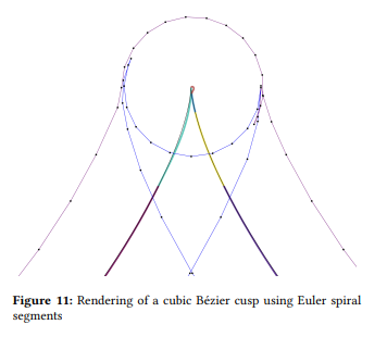
In practice, when rendering a cubic Bézier with a cusp, the region near the cusp is rendered with one Euler spiral segment approximately in shape of the top of a question mark, as shown in Figure 11. Its parallel curve is well defined, and has the correct shape for
ts outline of the stroke, given of course that the distance is within tolerance (as enforced by the error metric). As recommended in both Nehab [2020] and Kilgard [2020b], the rendering of a cusp with infinite curvature matches that of a near-cusp. The code to detect near-zero derivatives and re-evaluate is a small amount of non-divergent logic, unlike the additional “regularization” pass proposed in Section 3.1 of Nehab [2020] to handle special cases.
7.3.1 Cusps in parallel curves. Even when the input curve is smooth, its parallel curve contains a cusp when the (signed) curvature equals the offset distance (the half-width of the stroke). In published techniques, dealing with these cusps is a nontrivial effort, and involves numerical methods that are not GPU friendly. In particular, detecting locations in the cubic Bézier where the curvature crosses a given quantity is a medium-degree polynomial, and in general requires numerical techniques for root finding. In the approach of Nehab [2020], the root finder not only requires a hybrid Newton/bisection method, which requires iteration, but is also recursive in that it uses the roots of a polynomial of one degree lower as a subroutine. In general, polynomials up to cubic can be considered GPU-friendly, while finding cusps in cubic Béziers requires a higher degree.
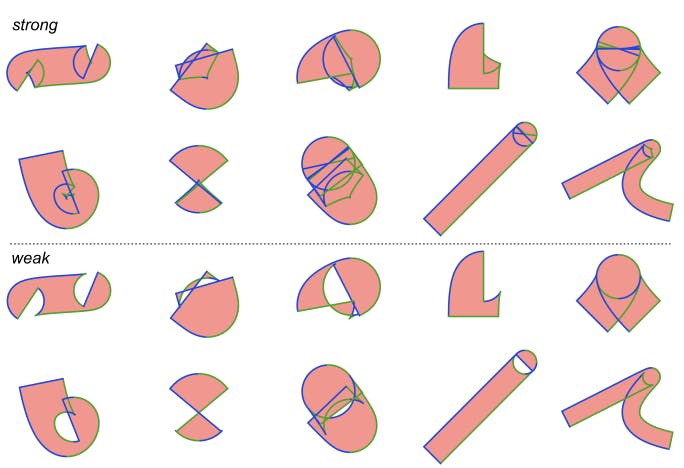
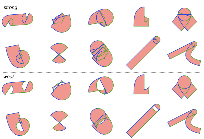
In the simplest case, weak stroke correctness with line segments as the output primitive, no additional work is needed – the flattening algorithm for Euler spiral parallel curves will naturally generate a point within the given error tolerance of the true cusp. However, generation of arc segments and drawing the evolutes needed for strong correctness both require subdivision at the parallel curve cusps. Fortunately, finding the cusp in the parallel curve of an Euler spiral is a simple linear equation, and there is at most one cusp in any such segment. Euler spirals are thus a good solution for determining cusps as a piecewise linear approximation to curvature
Authors:
This paper is