This paper is available on arxiv under CC 4.0 license.
Authors:
(1) Andrey Zhmoginov, Google Research & {azhmogin,sandler,mxv}@google.com;
(2) Mark Sandler, Google Research & {azhmogin,sandler,mxv}@google.com;
(3) Max Vladymyrov, Google Research & {azhmogin,sandler,mxv}@google.com.
Table of Links
- Abstract and Introduction
- Problem Setup and Related Work
- HyperTransformer
- Experiments
- Conclusion and References
- A Example of a Self-Attention Mechanism For Supervised Learning
- B Model Parameters
- C Additional Supervised Experiments
- D Dependence On Parameters and Ablation Studies
- E Attention Maps of Learned Transformer Models
- F Visualization of The Generated CNN Weights
- G Additional Tables and Figures
4 EXPERIMENTS
In this section, we present HYPERTRANSFORMER (HT) experimental results and discuss the implications of our empirical findings.

4.1 DATASETS AND SETUP
Datasets. For our experiments, we chose several most widely used few-shot datasets including OMNIGLOT, MINIIMAGENET and TIEREDIMAGENET. MINIIMAGENET contains a relatively small set of labels and is arguably the simplest to overfit to. Because of this and since in many recent publications MINIIMAGENET was replaced with a larger TIEREDIMAGENET dataset, we conduct many of our experiments and ablation studies using OMNIGLOT and TIEREDIMAGENET.
Models. HYPERTRANSFORMER can in principle generate arbitrarily large weight tensors by producing low-dimensional embeddings that can then be fed into another trainable model to generate the entire weight tensors. In this work, however, we limit our experiments to HT models that generate weight tensor slices encoding individual output channels directly. For the target models we focus on 4-layer CNN architectures identical to those used in MAML++ and numerous other papers. More precisely, we used a sequence of four 3 × 3 convolutional layers with the same number of output channels followed by batch normalization (BN) layers, nonlinearities and max-pooling stride-2 layers. All BN variables were learned and not generated. Experiments with generated BN variables did not show much difference with this simpler approach. Generating larger architectures such as RESNET and WIDERESNET will be the subject of our future work.
4.2 SUPERVISED RESULTS WITH LOGITS LAYER GENERATION
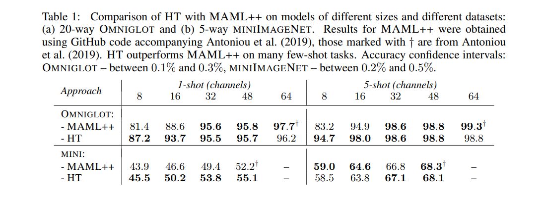
As discussed in Section 3.2, using a simple self-attention mechanism to generate the CNN logits layer can be a basis of a simple few-shot learning algorithm. Motivated by this observation, in our first experiments, we compared the proposed HT approach with MAML++ on OMNIGLOT and MINIIMAGENET datasets (see Table 1) with HT limited to generating only the final fully-connected logits layer.
In our experiments the dimensionality of local features was chosen to be the same as the number of model channels and the shared feature had a dimension of 32 regardless of the model size. The shared feature extractor was a simple 4-layer convolutional model with batch normalization and stride-2 3 × 3 convolutional kernels. Local feature extractors were two-layer convolutional models with outputs of both layers averaged over the spatial dimensions and concatenated to produce the final local feature. For all tasks except 5-shot MINIIMAGENET our transformer had 3 layers, used a simple sequence of encoder layers (Figure 2) and used the “output allocation” of weight slices (Section 3.1). Experiments with the encoder-decoder transformer architecture can be found in Appendix D. The 5-shot MINIIMAGENET results presented in Table 1 were obtained with a simplified transformer model that had 1 layer, and did not have the final fully-connected layer and nonlinearity. This proved necessary for reducing model overfitting of this smaller dataset. Other model parameters are described in detail in Appendix B.
Results obtained with our method in a few-shot setting (see Table 1) are frequently better than MAML++ results, especially on smaller models, which can be attributed to parameter disentanglement between the weight generator and the CNN model. While the improvement over MAML++

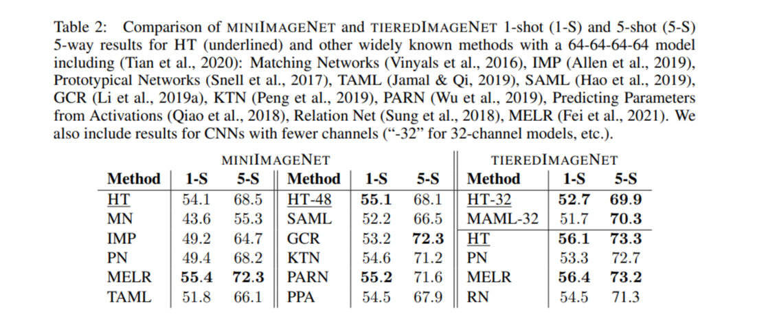
gets smaller with the growing size of the generated CNN, our results on MINIIMAGENET and TIEREDIMAGENET appear to be comparable to those obtained with numerous other methods (see Table 2). Discussion of additional comparisons to LGM-Net (Li et al., 2019b) and LEO (Rusu et al., 2019) using a different setup (which is why they could not be included in Table 2) and showing an almost identical performance can be found in Appendix C.
While the learned HT model could perform a relatively simple calculation on high-dimensional sample features, perhaps not too different from that in equation 1, our brief analysis of the parameters space (see Appendix D) shows that using simpler 1-layer transformers leads to a modest decrease of the test accuracy and a greater drop in the training accuracy for smaller models. However, in our experiments with 5-shot MINIIMAGENET dataset, which is generally more prone to overfitting, we observed that increasing the transformer model complexity improves the model training accuracy (on episodes that only use classes seen at the training time), but the test accuracy relying on classes unseen at the training time, generally degrades. We also observed that the results in Table 1 could be improved even further by increasing the feature sizes (see Appendix D), but we did not pursue an exhaustive optimization in the parameter space.
It is worth noting that overfitting characterized by a good performance on tasks composed of seen categories, but poor generalization to unseen categories, may still have practical applications. Specifically, if the actual task relies on classes seen at the training time, we can generate an accurate model customized to a particular task in a single pass without having to perform any SGD steps to fine-tune the model. This is useful if, for example, the client model needs to be adjusted to a particular set of known classes most widely used by this client. We also anticipate that with more complex data augmentations and additional synthetic tasks, more complex transformer based models can further improve their performance on the test set and a deeper analysis of such techniques will be the subject of our future work.
4.3 SEMI-SUPERVISED RESULTS
In our approach, the weight generation model is trained by optimizing the loss calculated on the query set and therefore any additional information about the task, including unlabeled samples, can be provided as a part of the support set to the weight generator without having to alter the optimization objective. This allows us to tackle a semi-supervised few-shot learning problem without making any substantial changes to the model or the training approach. In our implementation, we simply added unlabeled samples into the support set and marked them with an auxiliary learned “unlabeled” token ˆξ in place of the label encoding ξ(c).
Since OMNIGLOT is typically characterized by very high accuracies in the 97%-99% range, we conducted all our experiments with TIEREDIMAGENET. As shown in Table 3, adding unlabeled samples results in a substantial increase of the final test accuracy. Furthermore, notice that the model achieves its best performance when the number of transformer layers is greater than one.

This is consistent with the basic mechanism discussed in Section 3.2 that required two self attention layers to function.
It is worth noticing that adding more unlabeled samples into the support set makes our model more difficult to train and it gets stuck producing CNNs with essentially random outputs. Our solution was to introduce unlabeled samples incrementally during training. This was implemented by masking out some unlabeled samples in the beginning of the training and then gradually reducing the masking probability over time. In our experiments, we linearly interpolated the probability of ignoring an unlabeled sample from 0.7 to 0.0 in half the training steps.
4.4 GENERATING ADDITIONAL MODEL LAYERS
We demonstrated that HT model can outperform MAML++ on common few-shot learning datasets by generating just the last logits layer of the CNN model. But is it advantageous to be generating additional CNN layers (ultimately fully utilizing the capability of the HT model)?
We approached this question by conducting experiments, in which all or some layers were generated, while the remaining layers were learned as task-agnostic variables (usually the first few layers of the CNN). Our experimental results demonstrated a significant performance improvement due to the generation of the convolutional layers in addition to the CNN logits layer, but only for CNN models below a particular size. For OMNIGLOT dataset, we saw that both training and test accuracies for a 4- channel and a 6-channel CNNs increased with the number of generated layers (see Fig. 3 and Table 4 in Appendix) and using more complex transformer models with 2 or more encoder layers improved both training and test accuracies of fully-generated CNN models of this size (see Appendix D). However, as the size of the model increased and reached 8 channels, generating the last logits layer alone proved to be sufficient for getting the best results on OMNIGLOT and TIEREDIMAGENET. By separately training an “oracle” CNN model using all available data for a random set of n classes, we observed the gap between the training accuracy of the generated model and the oracle model (see Fig. 3), indicating that the transformer does not fully capture the dependence of the optimal CNN model weights on the support set samples. A hypothetical weight generator reaching maximum training accuracy could, in principle, memorize all training images being able to associate them with corresponding classes and then generate an optimal CNN model for a particular set of classes in the episode matching “oracle” model performance.
The positive effect of generating convolutional layers can also be observed in shallow models with large convolutional kernels and large strides where the model performance can be much more sensitive to a proper choice of model weights. For example, in a 16-channel model with two convolutional kernels of size 9 and the stride of 4, the overall test accuracy for a model generating only the final convolutional layer was about 1% lower than the accuracies of the models generating at least one additional convolutional filter. We also speculate that as the complexity of the task increases, generating some or all intermediate network layers should become more important for achieving optimal performance. Verifying this hypothesis and understanding the “boundary” in the model space between two regimes where a static backbone is sufficient or not will be the subject of our future work.

