This paper is available on arxiv under CC 4.0 license.
Authors:
(1) Marcin W ˛atorek, Faculty of Computer Science and Telecommunications, Cracow University of Technology, ul. Warszawska 24, 31-155 Kraków, Poland and [email protected] (M.W.);
(2) Jarosław Kwapie ´n, Complex Systems Theory Department, Institute of Nuclear Physics, Polish Academy of Sciences, Radzikowskiego 152, 31-342 Kraków, Poland and [email protected];
(3) Stanisław Drozd˙ z, Faculty of Computer Science and Telecommunications, Cracow University of Technology, ul. Warszawska 24, 31-155 Kraków, Poland, Complex Systems Theory Department, Institute of Nuclear Physics, Polish Academy of Sciences, Radzikowskiego 152, 31-342 Kraków, Poland and [email protected] (S.D.).
Table of Links
Abstract and Introduction
Data and Methodology
Results and Discussion
Conclusion and References
2. Data and Methodology
2.1. Data Sources and Preprocessing
In the present study, a data set of 24 financial time series representing contracts for difference (CFDs) from the Dukascopy trading platform [58] is considered. Unlike many other trading platforms, Dukascopy offers freely the high-frequency recordings of many financial instruments, which is the main reason it has been chosen as the data source. CFDs are characterised by the price movements that are close to the price movements of the original instruments, so we consider them as reliable proxies. Apart from the two highest capitalized cryptocurrencies, BTC and ETH, it includes the most important traditional financial instruments: 12 fiat currencies (Australian dollar—AUD, Canadian dollar—CAD, Swiss franc—CHF, Chinese yuan—CNH, euro—EUR, British-pound—GBP, Japanese yen—JPY, Mexican peso—MXN, Norwegian krone—NOK, New Zealand dollar—NZD, Polish zloty—PLN, and South African rand—ZAR), 4 commodities (WTI crude oil—CL, high grade copper—HG, silver—XAG, and gold—XAU), 4 US stock market indices (Nasdaq 100 NQ100, S&P500, Dow Jones Industrial Average—DJI, and Russell 2000—RUSSEL), German stock index—DAX 40—DAX, and the Japanese stock index—Nikkei 225—NIKKEI. All these instruments except for the non-US stock indices are expressed in USD (thus there is no USD in the data set) and their quotes cover a period from 1 January 2020 to 28 October 2022. Each week the quotes were recorded over the whole trading hours, i.e., from Sunday 22:00 to Friday 20:15 with a break between 20:15 and 22:00 each trading day (UTC) [58].
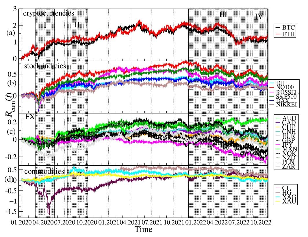
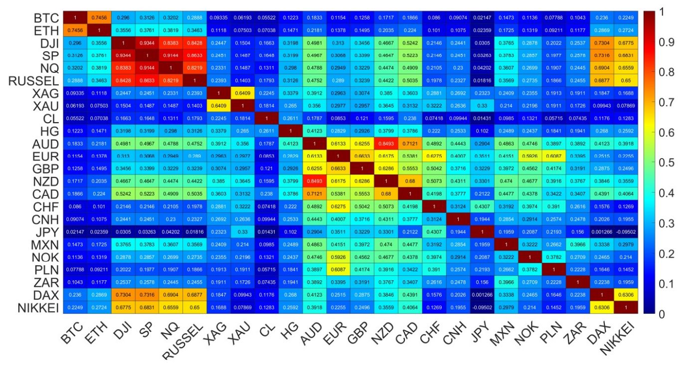
Cumulative log-returns of all the instruments considered are plotted in Figure 1 against time. The original price changes, sampled every ∆t = 10s, were transformed into logarithmic returns: r(tm) = ln Pi(tm+1) − ln Pi(tm), where Pi(tm) is a price quote recorded at time tm (m = 1, . . . , T) and i stands for a particular financial instrument. We use this particular time interval ∆t, because such a data set was available from the source. However, it is satisfactory because it allows us to avoid excessive null returns, which lower reliability of the detrended analysis (see below). In order to obtain the indicative relationships among all the time series, the Pearson correlation coefficient C [59] was calculated for the log-returns r(tm) from January to October 2022, when the joint bear market mentioned above was observed. A correlation matrix obtained for 24 financial instruments is shown in Figure 2. While the Pearson coefficient is one of the most widely applied measures of time series dependencies (and this is why we also exploited it in our study), the results obtained with it have to be taken with some reserve in our context. This is because the statistical tests that we carried out, i.e., the Jacque-Bera test for normality and the ARCH test for no heteroskedasticity, both rejected the respective null hypotheses with high confidence (p-value < 0.00001), which means that the data under study was both heavy-tailed and heteroskedastic. Obviously, such a result is not surprising, because fat tails of the return distributions and volatility clustering are well known effects observed in the financial time series [60–62]. Nevertheless, the very long time series that were analysed here and the statistical significance of the obtained results convinced us that the Pearson coefficient can still serve as an effective measure of the time series correlations even in such circumstances. Taking all this into account, a standard naming convention: small (0.1 ≤ C < 0.3), medium (0.3 ≤ C < 0.), and large (0.5 ≤ C ≤ 1.0) correlation was used to describe the coefficient values. The strongest cross-correlations (large, C > 0.6) can be seen for the stock indices, for BTC and ETH, for AUD, NZD and CAD, for XAU and XAG, and for EUR and GBP. If we consider the cross-correlations between BTC and the traditional instruments, the strongest ones can be seen for NQ100 and S&P500 (medium, C ≈ 0.32), DJI and RUSSEL (medium, C ≈ 0.29), DAX (small, C ≈ 0.24) and NIKKEI, (small C ≈ 0.23). The Pearson coefficient above 0.1 (small), is observed for BTC on the one side and HG, GBP and EUR, as well as the so-called commodity currencies: AUD, CAD, NZD, MXN, NOK, and ZAR, on the other side. The cross-correlations between ETH and the other instruments are even higher: C ≈ 0.38 (medium) for SP500 and NQ100, C ≈ 0.35 (medium) for DJI and RUSSEL, C ≈ 0.29 (medium) for DAX, and C ≈ 0.27 (small) for NIKKEI. The same is true for the cross-correlations between ETH and the commodity currencies: C ≈ 0.22 (small) for AUD, CAD, NZD, C ≈ 0.17 (small) for MXN, C ≈ 0.13 (small) for NOK, and C ≈ 0.12 (small) for ZAR. Among the commodities analyzed here, ETH is the most correlated with HG (C ≈ 0.15, small). The statistical significance of the coefficient values presented in Figure 2 has been checked by calculating the range: C¯ ± σC, where C¯ denotes mean and σC denotes standard deviation of C, from 100 independent realisations of the shuffled time series. The statistically insignificant correlation region is very close to 0 (the third decimal place), all the presented values, except DAX vs. JPY, are thus significant.


2.2. The q-Dependent Detrended Correlation Coefficient
Since the Pearson correlation coefficient as a measure has its drawbacks in the case of heavy tails, heteroskedasticity, and multi-scale nonstationarity (which are observed in the cryptocurrency market [9]) the cross-correlations will henceforth be determined using an alternative, better tailored method: the q-dependent detrended cross-correlation coefficient ρq(s) [63]. The detrended fluctuation analysis (DFA), which forms a basis for defining ρq(s), was developed with the intention to allow for detecting the long-range power-law autoand cross-correlations that produce trends on different time horizons [64]. Therefore, unlike more traditional methods of trend removal, both DFA and its derivative measures like the coefficient ρq(s) can successfully deal with nonstationarity on all scales [65]. ρq(s) enables, thus, considering the cross-correlation strength on different time scales and, if used in parallel with the multiscale DFA itself, is able to detect scale-free correlations. Moreover, owing to the parameter q, the correlation analysis can be focused on a specific range of the fluctuation amplitudes.
The steps to calculate ρq(s) are as follows. Two possibly nonstationary time series {x(i)}i=1,...,T and {y(i)}i=1,...,T of length T are divided into Ms boxes of length s starting from its opposite ends and integrated. In each box, the polynomial trend is removed:

where the polynomials P (m) of order m are applied. In this study m = 2 has been selected,
which performs well for the financial time series [66]. After this step 2Ms boxes are obtained in total with detrended signals. The next step is to calculate the variance and covariance for each
of the boxes ν:

where Z means X or Y. These quantities are used to calculate a family of the fluctuation functions of order q:

where a sign function sign f2 XY(s, ν)
is preserved in order to secure consistency of results for different qs.
The formula for the q-dependent detrended correlation coefficient is given as follows:

For q = 2 the above definition can be viewed as a detrended counterpart of the Pearson cross-correlation coefficient C [67]. The parameter q plays the role of a filter suppressing q < 2 or amplifying (q > 2) the fluctuation variance/covariance calculated in the boxes ν (see Eqs. (4) and (5)). For q < 2 boxes with small fluctuations contribute more to ρq(s), while for q > 2 the boxes with large fluctuations contribute more. Therefore, by using this measure, it is possible to distinguish the fluctuation size range that is a source of the observed correlations. In the numerical calculations below, we used our own software in which we implemented the algorithm described above.

