This paper is available on arxiv under CC 4.0 license.
Authors:
(1) Michael Günther, michael.guenther;
(2) Jackmin Ong, jackmin.ong;
(3) Isabelle Mohr, isabelle.mohr;
(4) Alaeddine Abdessalem, alaeddine.abdessalem;
(5) Tanguy Abel, tanguy.abel;
(6) Mohammad Kalim Akram, kalim.akram;
(7) Susana Guzman, susana.guzman;
(8) Georgios Mastrapas, georgios.mastrapas;
(9) Saba Sturua, saba.sturua;
(10) Bo Wang, bo.wang;
(11) Maximilian Werk, maximilian.werk;
(12) Nan Wang, nan.wang;
(13) Han Xiao, han.xiao}@jina.ai.
Table of Links
- Abstract & Introduction
- Related Work
- Training Process Overview
- Backbone Pre-training
- Fine-Tuning for Embeddings
- Evaluation
- Conclusion & References
- Appendix
5 Fine-Tuning for Embeddings
After pre-training the Jina BERT models, we further fin-tune each of the models to encode a text sequence into a single vector representation. The core idea behind our embedding approach is inspired by the Sentence-BERT technique [Reimers and Gurevych, 2019]. To enable a model to perform a text operation, we augment it with a mean pooling layer. This mean pooling step averages the token embeddings to merge their information into a single representation, without introducing additional trainable parameters. The training process for this enhanced model consists of an unsupervised phase followed by a supervised one.
5.1 First Unsupervised Fine-tuning
During the unsupervised fine-tuning phase, we train the models on a corpus of text pairs (q, p) ∈ Dpairs , comprising a query string q and a target string p.
Construction of the Text-Pair Datasets: We utilize roughly 40 diverse data sources, akin to the data preparation outlined in the report we previously published about our inaugural embedding model suite [Günther et al., 2023]. We observed that the inclusion of title-abstract pairs from documents significantly enhances performance on clustering tasks. As detailed in [Günther et al., 2023], we implement consistency filtering [Dai et al., 2023, Wang et al., 2022] to elevate the quality of the text pair corpus. For batch creation, we adhere to our earlier strategy: for every new batch, we randomly choose a data source and extract as many pairs as needed to fill that batch. All pairs within the data sources are pre-shuffled. Depending on the quality and quantity of the data sources, we assign different sampling rates for the pairs.
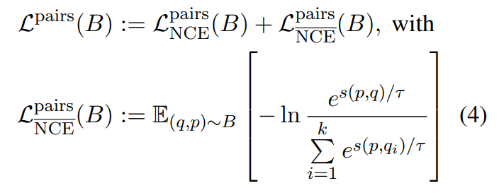
Training: The goal of unsupervised fine-tuning is to encode text values that constitute a pair into analogous embedding representations, while encoding texts that aren’t paired into distinct embeddings. To achieve this contrastive goal, we employ the InfoNCE [van den Oord et al., 2018] loss function, similar to our earlier embedding models [Günther et al., 2023]. This loss function calculates the loss value for a pair (q, p) ∼ B within a batch B ∈ Dk of k text pairs as follows:

The function evaluates the cosine similarity s(p, q) between a given query q and its corresponding target p, relative to the similarity of all other targets in the batch. Given the typically symmetric nature of similarity measures, we compute the loss in both directions:

The constant temperature parameter τ influences how the loss function weighs minor differences in the similarity scores [Wang and Liu, 2021]. Empirical testing suggests that τ = 0.05 is effective.
5.2 Second Supervised Fine-tuning
The goal of the supervised fine-tuning stage is to improve the models’ ranking capabilities. This improvement is achieved by training with datasets that include additional negative examples.
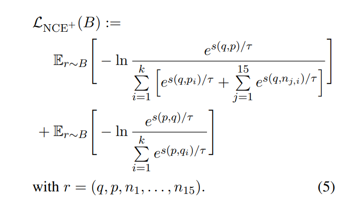
Dataset with annotated negatives: We have prepared retrieval datasets, such as MSMarco [Bajaj et al., 2016] and Natural Questions (NQ) [Kwiatkowski et al., 2019], in addition to multiple non-retrieval datasets like the Natural Language Inference (NLI) dataset [Bowman et al., 2015]. These datasets encompass a collection of queries with annotated relevant passages and several negative examples, consistent with earlier work [Wang et al., 2022]. Each training batch B, structured as (q, p, n1, . . . , n15), includes one positive and 15 negative instances. For retrieval datasets, hard negatives are discerned by identifying passages deemed similar by retrieval models. This approach instructs the model to prioritize relevant documents over those that are merely semantically related. For non-retrieval datasets, negatives are selected randomly, since drawing a clear line between positives and hard negatives isn’t feasible. This is because, unlike relevancy, it’s challenging to make a binary determination regarding the similarity or dissimilarity of two textual values. Consequently, opting for hard negatives in such datasets seemed to diminish the models’ quality. Nonetheless, it remains crucial to integrate these datasets into the stage III training to ensure continued performance on non-retrieval tasks. To ensure that hard negative passages are indeed less relevant than the annotated relevant ones, we employ a cross-encoder model to validate that their relevance score is indeed lower.
Training: Our training employs a modified variant of the InfoNCE loss function, denoted as LNCE+ and described by Equation (5). Similar to the preceding loss function, this one is bidirectional and incorporates the additional negatives when pairing queries with passages:

5.3 Memory Optimizations
When training embedding models, having a large batch size is crucial. This is because the InfoNCE loss functions L pairs and LNCE+ compute the loss values based on the entirety of the batch. The batch size determines the number of text values each individual text value is compared against. As a result, the computed loss value might not be as expressive with smaller batches. Li et al. [2023] provided an in-depth analysis, highlighting the positive impact of larger batch sizes on the performance of the resultant embedding model. To accommodate larger batch sizes, it becomes essential to minimize the memory overhead during training. We achieved this by training our models in mixed precision [Micikevicius et al., 2018] and leveraging the deepspeed [Rasley et al., 2020] framework for further optimization. Activation checkpointing [Chen et al., 2016] was also employed to curtail memory usage. Specifically, we inserted a checkpoint after each BERT layer within our model.

