Authors:
(1) Ruohan Zhang, Department of Computer Science, Stanford University, Institute for Human-Centered AI (HAI), Stanford University & Equally contributed; [email protected];
(2) Sharon Lee, Department of Computer Science, Stanford University & Equally contributed; [email protected];
(3) Minjune Hwang, Department of Computer Science, Stanford University & Equally contributed; [email protected];
(4) Ayano Hiranaka, Department of Mechanical Engineering, Stanford University & Equally contributed; [email protected];
(5) Chen Wang, Department of Computer Science, Stanford University;
(6) Wensi Ai, Department of Computer Science, Stanford University;
(7) Jin Jie Ryan Tan, Department of Computer Science, Stanford University;
(8) Shreya Gupta, Department of Computer Science, Stanford University;
(9) Yilun Hao, Department of Computer Science, Stanford University;
(10) Ruohan Gao, Department of Computer Science, Stanford University;
(11) Anthony Norcia, Department of Psychology, Stanford University
(12) Li Fei-Fei, 1Department of Computer Science, Stanford University & Institute for Human-Centered AI (HAI), Stanford University;
(13) Jiajun Wu, Department of Computer Science, Stanford University & Institute for Human-Centered AI (HAI), Stanford University.
Table of Links
Brain-Robot Interface (BRI): Background
Conclusion, Limitations, and Ethical Concerns
Appendix 1: Questions and Answers about NOIR
Appendix 2: Comparison between Different Brain Recording Devices
Appendix 5: Experimental Procedure
Appendix 6: Decoding Algorithms Details
Appendix 7: Robot Learning Algorithm Details
Appendix 6: Decoding Algorithms Details
For both SSVEP and MI, we select a subset of channels and discard the signals from the rest, as shown in Figure 6. They correspond to the visual cortex for SSVEP, and the motor and visual areas for MI (with peripheral areas). For muscle tension (jaw clenching), we retain all channels.
SSVEP. To predict the object of interest, we apply Canonical Correlation Analysis (CCA) as shown in [77] to the collected SSVEP data. As each potential object of interest is flashing at a different frequency, we are able to generate reference signals Yfn for each frequency fi:

where fs is the sampling frequency and Ns is the number of samples.

By calculating the maximum correlation ρfn for each frequency fn used for potential objects of interest, we are then able to predict the output class by finding argmaxfn (ρfn ) and matching the result to the object of interest with that frequency.
Furthermore, we are able to return a list of predicted objects of interest in descending order of likelihood by matching each object to a list of descending maximum correlations ρfn.
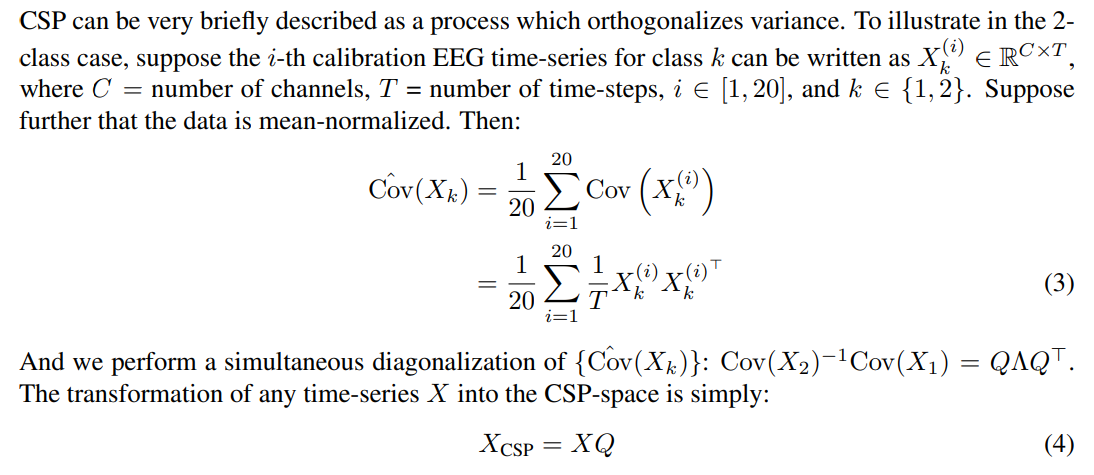
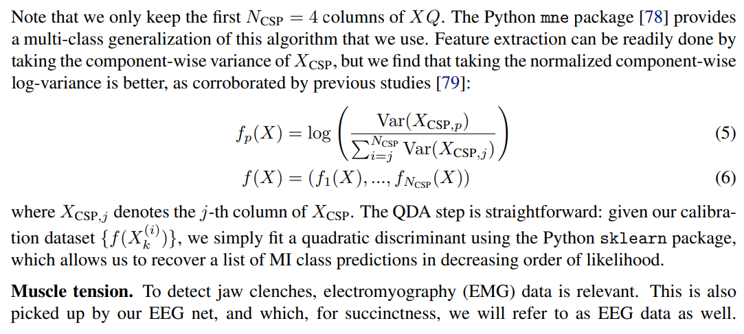
Motor imagery. To perform MI classification, we first band-pass filter the data between 8Hz - 30Hz, as that is the frequency range that includes the µ-band and β-band signals relevant to MI. The data is then transformed using the Common Spatial Pattern (CSP) algorithm. CSP is a linear transformation technique that applies a rotation to the data to orthogonalize the components where the over-timestep variance of the data differs the most across classes. We can then use the logvariance of each time series after rotation as features and perform QDA. Thereafter, we extract features by taking the normalized variance of this transformed data (called “CSP-space data”). We then perform Quadratic Discriminant Analysis (QDA) on this data. To calculate our calibration accuracy, we perform K-fold cross validation with KCV = 4, but we use the entire calibrate dataset to fit the classifier for deployment at task-time.


Facial muscle tension results in a very significant high-variance signal across almost all channels that is very detectable using simple variance-based threshold filters without having to perform any frequency filters. Recall that we record three 500ms-long trials for each class (“Rest”, “Clench”). In short, for each of the calibration time-series, we take the variance of the channel with the median variance; call this variance m. Then, we just take the mid-point between the maximum m between the rest samples, and the minimum m between the clench samples, and have this be our threshold variance level.

This paper is available on arxiv under CC 4.0 license.

