This paper is available on arxiv under CC 4.0 license.
Authors:
(1) Jihoon Chung;
(2) Zhenyu (James) Kong.
Table of Links
- Abstract & Introduction
- Review of Related Work
- Proposed Research Methodology
- Numerical Case Studies
- Real-World Simulation Case Studies
- Conclusion
- References
V. REAL-WORLD SIMULATION CASE STUDIES
An assembly operation from an actual auto-body assembly process is used as a real-world case study. Fig. 5 describes a car’s floor pan, which is the assembled product from this process. The assembled product consists of four parts, including the right bracket, left bracket, right floor pan, and left floor pan. Fig. 6 shows the process assembly procedure consisting of three stations. During the assembly process, the parts are held by fixtures, which are the KCCs in this process [7]. KPCs are measured from four points, namely, M1, M2, M3, and M4, respectively, as shown in Fig. 5. Every part has a designated location for measuring the KPCs. For instance, part 1 has M1, part 2 has M2, part 3 has M3, and part 4 has M4. These measurements can be taken at each station once the relevant part has been assembled in the preceding stations. For example, M3 on part 3 cannot be measured in station 1 because part 3 has not yet been assembled at station 1 [7]. In the designated location, KPCs are measured in three directions (X, Y, and Z). In this assembly process, there exists a total of 33 KCCs, which are dimensional errors of fixture
![Fig. 5. Floor-pan assembly model [5].](https://cdn.hackernoon.com/images/fWZa4tUiBGemnqQfBGgCPf9594N2-1x83s05.jpeg)
locators [8]. The fault pattern matrix Φ is established based on the literature [7], [11], [47] and provided in Appendix F. Since the number of measurements (12) is less than that of KCCs (33), it causes an underdetermined system in the fault quality linear model. Therefore, sparse estimation is required to identify process faults.
![Fig. 6. Floor-pan assembly model from three assembly stations. [5].](https://cdn.hackernoon.com/images/fWZa4tUiBGemnqQfBGgCPf9594N2-l393s01.jpeg)
In this assembly process, two lists of correlated KCCs exist; the rest are assumed to be independent [8]. The first list comprises six KCCs, including KCC8, KCC9, KCC10, KCC11, KCC12, and KCC13. The second list is composed of KCC31, KCC32, and KCC33. The correlation structures of the two groups are described (for simplification, the lower triangular terms are removed) as follows [8]:


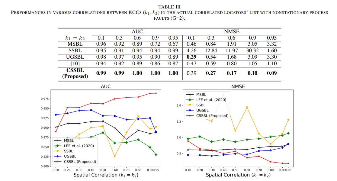
To provide nonstationary process faults along the KPCs samples collected over time, two groups are provided. In the first group, the first correlated list is provided as process faults. For the process faults of the second group, all the correlated lists and one independent KCCs are included. Therefore, the case study represents the situation when the process faults evolve over time since the variation of certain KCCs will be propagated to other KCCs if the process faults are not mitigated immediately during the process. 50 KPCs samples are generated from each group. The variances of process faults, non-process faults, and noise of KPCs are determined to be the same value as in Section IV. In addition, performance evaluation measures and benchmark methods used in Section IV are still utilized in Section V. Table III shows the performance comparison in AUC and NMSE by varying the correlation coefficients. For convenience, the correlation coefficients k1 and k2 are equal and are selected from {0.1, 0.3, 0.6, 0.9, 0.95} in the case studies. Specifically, the AUC of the proposed method is close to 1.0 at every correlations levels, representing the perfect classification between the process faults and non-process faults in terms of estimated variance. The effectiveness of the proposed method is significant in NMSE when a high correlation exists. Specifically, the NMSE of the proposed method is less than 10% of that of all the benchmark methods when the correlation coefficient is 0.9 and 0.95.
To demonstrate the generalizability of the proposed method, the correlated KCCs are randomly selected in further case studies. Assuming there exist two correlated lists with the size of three, respectively. Therefore, six KCCs are randomly selected from 33 KCCs for two correlated lists in each trial. As in the previous study, one correlated list is provided as process faults in the first group, while two correlated lists and two independent KCCs are used as process faults in the remaining second group. Fig. 7 shows the performances of all the methods in AUC and NMSE results in ten different spatial correlations (i.e., k1 = k2). From Fig. 7 (a), it is prominent that the proposed method successfully differentiates between process faults and non-process faults. Specifically, the AUC of the proposed method is nearly 1.0, while those of most benchmark methods are below 0.9 in the highly correlated case studies. In addition, Fig. 7 (b) represents that the proposed method provides valuable information to the practitioners to determine when to stop the operations to maintain the process when a high correlation exists between KCCs. All the benchmark methods illustrate similar trends compared to Section IV since the methods cannot consider both the spatial correlation of KCCs and the nonstationary process faults.

