Authors:
(1) Jonathan H. Rystrøm.
Table of Links
B Other Models
B.1 Model without activity-level

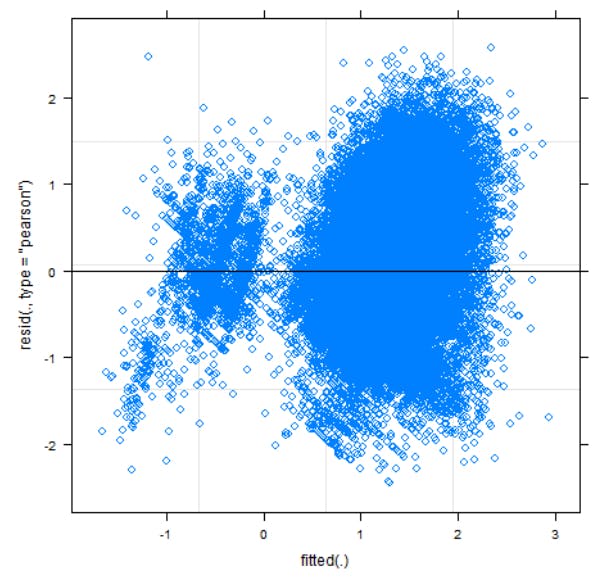
However, when we ran the model (also using lmerTest (Kuznetsova et al., 2017)) and plotted the residuals, we got the following:

Just from a brief visual inspection, it is clear to see that the residuals are not randomly distributed: There are two distinct ”bands” that both seem to trend upward. This breaks the assumption that the residuals are randomly distributed (Poole & O’Farrell, 1971). While many assumption violations are reduced with enough data (Baayen et al., 2008; Schielzeth et al., 2020), non-linearity is not one of them (Poole & O’Farrell, 1971).
Fortunately, the non-random residuals were (partially) fixed by introducing activity-level for the reasons described in section 3.3.
B.2 Problematic Categories Removed
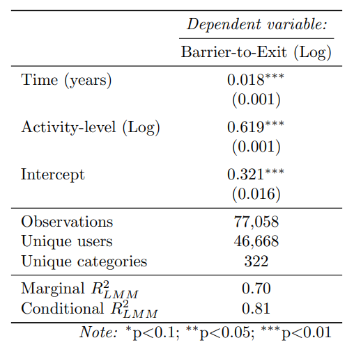
Here we fit the main model (eq. 5, with problematic categories removed. We define a problematic category as a category with a fitted random effect of less than -0.5. We obtain this threshold by visually inspecting Fig. 7.
The results of this fit can be seen below in 2:


B.3 Gamma mixed-effects model
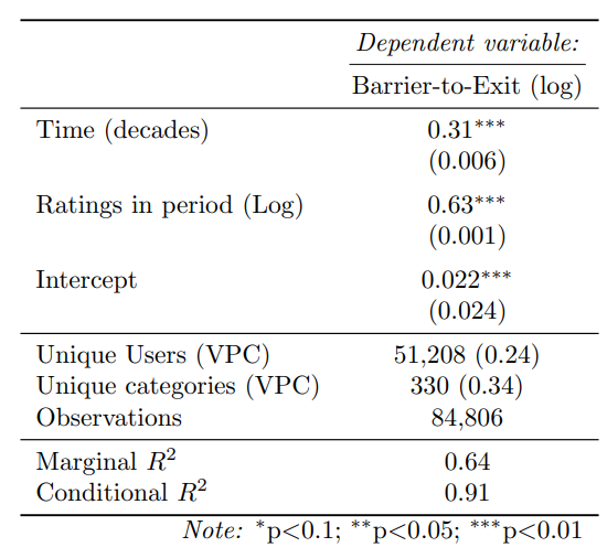
In the following, we refit the main model (eq. 5) using a Gamma regression. This is the most widely recommended solution in the literature on fitting right-tailed, heteroscedastic outcomes (Feng et al., 2014; Villadsen & Wulff, 2021).
However, since we discovered this after running our initial models, we could only justify doing this as a post-hoc test.
I use the lme4-package to fit the model (Bates et al., 2014). To avoid convergence errors and adapt the model to the formula, we make the following alterations:
-
Add a gamma log-link function (Fox, 2015)
-
change the year (β1) estimate to decades. This has the effect of rescaling the effect size.
-
We still log-transform the activity-level to rescale it. As this is not part of the hypothesis, this does not affect our interpretation.


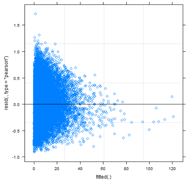
This leads us to the interpretation. The effect size per decade is 0.31, which is highly significant (SE=0.006, T=24, p ≪ 0.001). This translates into 34% increase per decade or 3% increase per year. This is the same direction as our transformed linear model, with somewhat larger results. However, as these come from an almost unidentifiable fit with extremely non-random residuals, no inferences can be drawn from this.
Some of this indicates that the conditional distribution of Barrier-to-Exit is not a Gamma distribution. Pursuing the GLMM path would require further assessments of the best-fitting distribution. This could be by e.g. applying the Box-Cox method as described by Villadsen and Wulff (2021).
This paper is available on arxiv under CC 4.0 license.

