Authors:
(1) Jonathan H. Rystrøm.
Table of Links
A Validation of Assumptions
There are several assumptions to validate for crossed-linear mixed effects models (Baayen et al., 2008). Specifically, we need to assess:
• Linearity: Is the phenomenon the model captures actually linear? This can be tested by looking for trends in the residuals. If no trends are found, linearity holds (Poole & O’Farrell, 1971).
• Homogeneity of Variance: Is the variance across residuals equal? This can be tested by plotting residuals against response and looking for cone-like shapes (Fox, 2015).
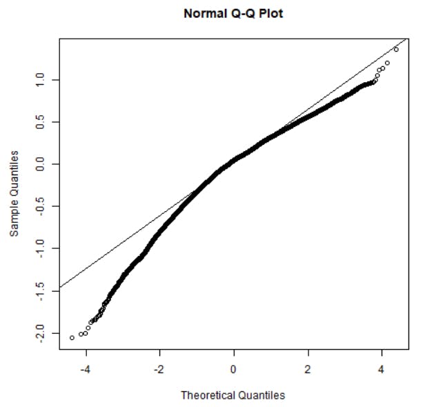
• Normality of residuals: Are the residuals normally distributed? We can assess this by a QQ-plot over the residuals.
• Normality of random effects: Per the definition of crossed-effects mixed effects models (Baayen et al., 2008), we expect the residuals to be normal. This can be assessed similarly to the random effects.
Note that testing the assumptions relies on visual tests rather than statistical tests. This is not for a lack of statistical tests (see e.g. Fox, 2015). Rather it is because statistical tests tend to become oversensitive for large datasets (Ghasemi & Zahediasl, 2012). Given our dataset has more than 50,000 observations, it is safer to use visual tests.
First, let us test for linearity and heteroscedasticity. The residual plot can be seen in fig. 5:
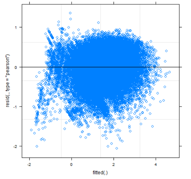
At first glance, there seems to be no strong heteroscedasticity or apparent linearity. However, at a closer look, there are some weird outliers in the bottom left corner. Furthermore, there is a weird kind of straight line going from the top left corner and down towards the middle. This indicates that there may be something wrong with the model.
Let us now assess the normality of the residuals:
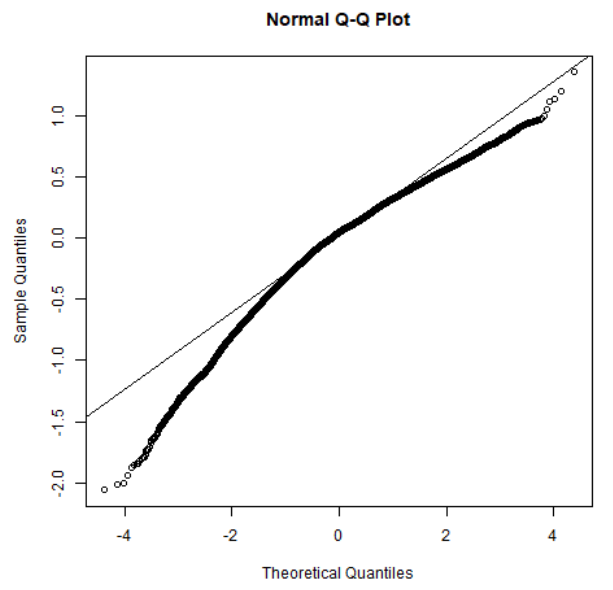
We notice that the residuals are generally lower than the normality line. This indicates a left skew in the residuals, i.e. there are smaller outliers. While the fixed effects are robust against this type of skew, the estimates for group-level variances are more affected (Schielzeth et al., 2020).
Finally, let us consider the normality of the random effects. A qq-plot of the random effects for the two levels can be seen below:
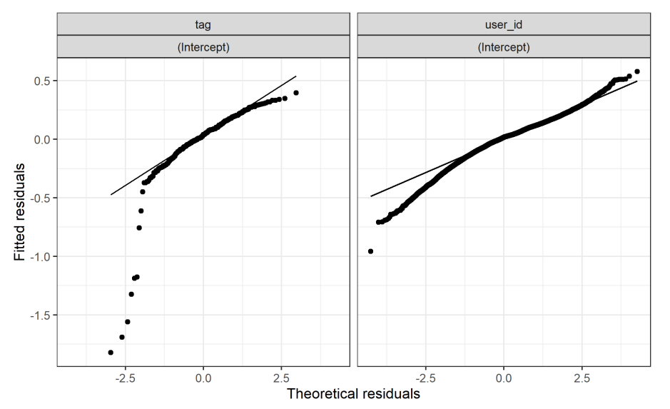
Here we see a dramatic skew toward the lower level of the fitted residuals. This implies that there are weird dynamics in the lower values of Barrier-to-Exit.
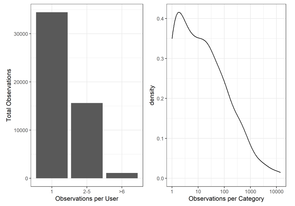
Part of this may be because of the relatively few observations per user (see fig 8). This highlights another issue with measuring Barrier-to-Exit across time: because it requires many observations over a long period of time to calculate sufficient precision of revealed preferences, it’s hard to measure changes on the individual level.
While the effects of non-normality on the fixed effects should be minor (Schielzeth et al., 2020), we nevertheless conduct a robustness check. In the robustness check, we remove the problematic categories and refit the main model (eq. 5). The results of this can be seen in Appendix B.2
This paper is available on arxiv under CC 4.0 license.

