How to Approximate Curves Using Bézier and Euler Spiral Segments

Table Of Links

ABSTRACT

1 INTRODUCTION

2 FLATTENING AND ARC APPROXIMATION OF CURVES

3 EULER SPIRALS AND THEIR PARALLEL CURVES

4 FLATTENED PARALLEL CURVES

5 ERROR METRICS FOR APPROXIMATION BY ARCS

6 EVOLUTES

7 CONVERSION FROM CUBIC BÉZIERS TO EULER SPIRALS

8 GPU IMPLEMENTATION

9 RESULTS

CONCLUSIONS, FUTURE WORK AND REFERENCES

FLATTENING AND ARC APPROXIMATION OF CURVES

The core problem in stroke expansion is approximating the desired curve by segments of some other curve, usually a simpler one. These segments must be within an error tolerance of the source curve, and ideally close to a minimal number of them. We consider a number of source-to-target pairs, most importantly cubic Béziers to Euler spirals, and Euler spiral parallel curves to either lines or arcs.

There are generally three approaches to such curve approximation. The most straightforward but also least efficient is “cut then measure,” usually combined with adaptive subdivision. In this technique, a candidate approximate curve is produced, then the error is measured against the source curve, usually by sampling a number of points along both curves and determining a maximum error (or perhaps some other error norm). If the error is within tolerance, the approximation is accepted.

Otherwise, the curve is subdivided (usually at 𝑡 = 0.5) and each half is recursively approximated. A substantial fraction of all curve approximation methods in the literature are of this form, including Nehab [2020]. The main disadvantage is the cost of computing the error metric. Another risk is underestimating the error due to inadequate sampling; this is a particular problem when the source curve contains a cusp. The next approach is similar, but uses an error metric to estimate the error.

Ideally such a metric is a closed-form computation rather than requiring iteration. A good error metric is conservative, yet tight, in that it never underestimates the error (which would allow results exceeding the error bound to slip through), and does not significantly overestimate the error, which would result in more subdivision than optimal. By far the most efficient approach is an invertible error metric.

In this approach, the error metric has an analytic inverse, or at least a good numerical approximation. Because the metric is invertible, it can predict the number of subdivisions needed, as well as the parameter value for each subdivision. If the error metric is accurate, then approximation is near-optimal.

One example of an invertible error metric is angle step, used in polar stroking (Kilgard [2020b]); the number of subdivisions is the total angle subsumed by the curve divided by the angle step size, and the parameter value for each subdivision is the result of solving for a tangent direction. Another widely used invertible error metric is Wang’s formula (Goldman [2003], Section 5.6.3), which gives a bound on the flattening error based on the second derivative of the curve.

This metric is conservative but works well in practice; among other applications, it is used in Skia for path flattening. The chief limitation of Wang’s method is that it computes a subdivision bound for a Bézier curve without accounting for the displacement of the parallel curve due to stroking. When applied naively to generation of parallel curves, it can undershoot substantially, especially near cusps.

2.1 Error metrics for flattening

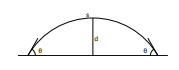
The distance between a circular arc segment of length 𝑠 and its chord, with angle between arc and chord of 𝜃 (see Figure 3), is exactly (1−cos 𝜃) 𝑠 2𝜃 . The curvature is 𝜅 = 2𝜃 𝑠 (equivalently, 𝜃 = 𝜅𝑠 2 ), and this remains constant even as the arc is subdivided. Rewriting, 𝑑 = (1 − cos 𝜅𝑠 2 ) 1 𝜅 . From this, we can derive a precise, invertible error metric. Subdividing the arc into 𝑛 segments, the distance error for each segment is 1 𝜅 (1 − cos 𝜅𝑠 2𝑛 ). Solving for 𝑛, we get:

                                                        𝑛 = 𝑠𝜅 2 cos−1 (1 − 𝑑𝜅) 

To flatten a finite arc, round up 𝑛 to the nearest integer. This will cause the error to decrease, so will still be within the error bounds. Note that the number of subdivisions is proportional to the arc length. Another way of stating this relationship is that the subdivision density, the number of subdivisions per unit of arc length, is constant. The error metric for flattening an arc is exact. It always yields the minimum number of subdivisions needed to flatten the curve, and the flattening error is the least possible given that number of subdivisions.

For general curves, an exact error bound is not feasible, and we resort to an approximation. Again the circular arc provides a good example. Applying the small angle approximation cos 𝜃 ≈ 1 −𝜃 2 /2, the approximate distance error is 𝑑 = 𝜅𝑠2 8𝑛 2 , and solving for 𝑛 we get 𝑛 = 𝑠 √︃ 𝜅 8𝑑 . Note that this estimate is conservative, in that it will always request more subdivision and thus produce a lower error than the exact metric.

We are of course concerned with the flattening of more general curves (ultimately the parallel curve of a cubic Bézier), not simply circular arcs, so the curvature is not constant. An obvious approach to try would be to use the maximum error. This would be conservative with respect to error tolerance, but also generate too much subdivision when the curve has a small region of high curvature. In the limit, the curve can contain a cusp of infinite curvature, which would entail infinite subdivision.

Similarly, sampling the curvature at a single point can either underestimate or overestimate the error. The ideal approach would be a form of average curvature that is tractable to compute, and accurately predicts the flattening error. To that end, we propose the following error metric to estimate the maximum distance between an arbitrary curve of length 𝑠ˆ and its chord.

                                                                𝑑 ≈ 1 8 ∫ 𝑠ˆ 0 √︁ |𝜅(𝑠)|𝑑𝑠!2 

This formula is the same as the approximate error metric for circular arcs, except that instead of a constant curvature value, a norm-like average with an exponent of 1/2 is used (it is not considered a true norm because the triangle inequality does not hold). This particular formulation has two strong advantages. First, it has been empirically validated to accurately predict the distance between chord and curve for a variety of curves.

In particular, we believe that when curvature is monotonic, it is a tight bound both above and below (and later we will see that in our algorithm it is always evaluated on curve segments with such monotonic curvature). Second, this formula lends itself to invertible error metrics. This formula also has a meaningful interpretation: the quantity under the integral sign is the subdivision density, and represents the number of subdivisions per unit length of an optimal flattening as the error tolerance approaches zero. In particular, the number of subdivisions is:

                                                       𝑛 = ∫ 𝑠ˆ 0 √︁ |𝜅(𝑠)|𝑑𝑠! √︂ 1 8�

In addition, if the function represented by the integral is invertible, then the corresponding error metric is invertible. Evaluate the function to determine the number of subdivision points, then evenly divide the result, using the inverse of the function to map these values back into parameter values for the source curve being approximated.

2.2 Error metrics for flattening Euler spirals

We choose Euler spiral segments for our intermediate curve representation precisely because their simple formulation in terms of curvature (Cesàro equation) results in similarly simple subdivision density integrals. An Euler spiral segment is defined by 𝜅(𝑠) = 𝑎𝑠 + 𝑏, or alternatively 𝜅(𝑠) = 𝑎(𝑠 − 𝑠0), where 𝑠0 = −𝑏/𝑎 is the location of the inflection point.

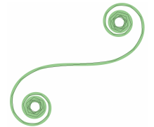
Applying the above error metric, the subdivision density is simply √︁ |𝑎(𝑠 − 𝑠0)|. The integral is 2 3 √ 𝑎(𝑠 −𝑠0) 1.5 , which is readily invertible. An immediate consequence is that flattening an Euler spiral by choosing subdivision points 𝑠𝑖 = 𝑎 · 𝑖 2 3 produces a near-optimal flattening, as visualized in Figure 4.