
Table Of Links
2 FLATTENING AND ARC APPROXIMATION OF CURVES
3 EULER SPIRALS AND THEIR PARALLEL CURVES
5 ERROR METRICS FOR APPROXIMATION BY ARCS
7 CONVERSION FROM CUBIC BÉZIERS TO EULER SPIRALS
CONCLUSIONS, FUTURE WORK AND REFERENCES
EULER SPIRALS AND THEIR PARALLEL CURVES
It is common to approximate cubic Béziers to some intermediate curve format more conducive to offsetting and flattening. A number of published solutions (Yzerman [2020], Nehab [2020]) use quadratic Béziers, as it is well suited for computation of parallel curves. Even so, this curve has some disadvantages. For one, it cannot model an inflection point, so the source curve must be subdivided at inflection points. Like these other approaches, we also use an intermediate curve, but our choice is an Euler spiral.
In some ways it is similar to quadratic Béziers – it also has 𝑂(𝑛 4 ) scaling and is best computed using geometric Hermite interpolation – but differs in others. It has no difficulty modeling an inflection point. Further, its parallel curve has a particularly simple mathematical definition and clean behavior regarding cusps.
An Euler spiral segment is defined as having curvature linear in arc length. The parallel curve of the Euler spiral (also known as “clothoid”) was characterized by Wieleitner [1907] well over a hundred years ago, and has a straightforward closed-form Cesàro representation, curvature as a function of arc length, of the form 𝜅(𝑠) = 𝑐0 (𝑠 − 𝑠0) −1/2+𝑐1.
Euler spirals as an intermediate curve representation for computing parallel curves was proposed in Levien [2021], which also expands on the Wieleitner reference (including an English translation) and Cesàro equation.
FLATTENED PARALLEL CURVES
The geometry of a stroke outline consists of joins, caps, and the two parallel curves on either side of the input path segments, offset by the half linewidth. The joins and caps are not particularly difficult to calculate, but parallel curves of cubic Béziers are notoriously tricky [11]. Analytically, it is a tenth order algebraic curve, which is not particularly feasible to compute directly.
Conceptually, generating a flattened stroke outline consists of computing the parallel curve of the input curve segment followed by flattening, the generation of a polyline that approximates the parallel curve with sufficient accuracy (which can be measured as Fréchet distance). However, these two stages can be fused for additional performance, obviating the need to store a representation of the intermediate curve.
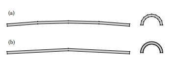
Using a subpixel Fréchet distance bound guarantees that the rendered image does not deviate visibly from the exact rendering. Another choice would be uniform steps in tangent angle, as chosen by polar stroking [12]. However, at small curvature, the stroked path can be off by several pixels, and at large curvature there may be considerably more subdivision than needed for faithful rendering. The limitation of the angle step error metric is shown in Figure 5.
The top row shows the use of a distance-based error metric, as is used in our approach, which is visually consistent at varying curvature (in practice, a tolerance value of 0.25 of a pixel is below the threshold of perceptibility). The bottom row shows a consistent angle step, as implemented in polar stroking, but has excessive distance error at low curvature, and excessive subdivision at high curvature. It should be noted, to avoid the undershoot at low curvature, both the Skia [8] and Rive [9] renderers use a hybrid of the Wang and polar stroking error metrics.
4.1 The subdivision density integral
The subdivision density for the parallel curve of an Euler spiral, normalized so that its inflection point is at −1 and the cusp of the
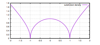
parallel curve is at 1, is simply √︁ |1 − 𝑠 2 |. This function is plotted in Figure 6. The subdivision density integral for the parallel curve of an Euler spiral is given as follows:
𝑓 (𝑥) = ∫ 𝑥 0 √︁ |𝑢 2 − 1|𝑑𝑢
This integral has a closed-form analytic solution:
𝑓 (𝑥) = ( 1 2 (𝑥 √︁ |𝑥 2 − 1| + sin−1 𝑥) if |𝑥 | ≤ 1 1 2 (𝑥 √︁ |𝑥 2 − 1| − cosh−1 𝑥 + 𝜋 4 ) if 𝑥 ≥ 1
Values for 𝑥 < −1 follow from the odd symmetry of the function.
4.2 Approximation of the subdivision density integral
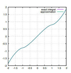
The subdivision density integral (Section 4.1) is fairly straightforward to compute in the forward direction, but not invertible using a straightforward closed-form equation. Numerical techniques are possible, but require multiple iterations to achieve sufficient accuracy, so are slower. In this subsection, we present a straightforward and accurate approximation, constructed piecewise from easily invertible functions.
This approximation was found empirically, by interactively tuning candidate approximation functions in the Desmos graphing calculator. The exact integral and the approximation are shown in Figure 7. Visually, it is clear that the agreement is close. We also built a test suite (included in our supplemental materials) to exhaustively test the subdivision count using a property testing approach, finding that the worst case discrepancy between approximate and exact results is 6%.
If higher flattening quality is desired at the expense of slower computation, this approximation could be used to determine a good initial value for numeric techniques; two iterations of Newton solving are enough to refine this guess to within 32-bit floating point accuracy. The approximation is as follows:
𝑓approx (𝑥) = sin𝑐1𝑥 𝑐1 if 𝑥 < 0.8 √ 8 3 (𝑥 − 1) 1.5 + 𝜋 4
                                                                    if 0.8 ≤ 𝑥 < 1.25 0.6406𝑥 2 − 0.81𝑥 + 𝑐2

                                                                    if 1.25 ≤ 𝑥 < 2.1 0.5𝑥 2 − 0.156𝑥 + 𝑐3

                                                                    if 𝑥 ≥ 2.1
𝑐1 = 1.0976991822760038
𝑐2 = 0.9148117935952064
𝑐3 = 0.16145779359520596
The primary rationale for the constants is for the approximation to be continuous. The other parameters were determined empirically; further automated optimization is possible but is unlikely to result in dramatic improvement. Further, this approximation is given for positive values. Negative values follow by symmetry, as the function is odd.
Authors:
This paper is