This paper is available on arxiv under CC BY-SA 4.0 DEED license.
Authors:
(1) Lana L. Blaschke, Earth System Modelling, School of Engineering and Design, Technical University of Munich, Munich, Germany, Potsdam Institute for Climate Impact Research, Potsdam, Germany and [email protected];
(2) Da Nian, Potsdam Institute for Climate Impact Research, Potsdam, Germany;
(3) Sebastian Bathiany, Earth System Modelling, School of Engineering and Design, Technical University of Munich, Munich, Germany, and Potsdam Institute for Climate Impact Research, Potsdam, Germany;
(4) Maya Ben-Yami, Earth System Modelling, School of Engineering and Design, Technical University of Munich, Munich, Germany, and Potsdam Institute for Climate Impact Research, Potsdam, Germany;
(5) Taylor Smith, Institute of Geosciences, University of Potsdam, 14476 Potsdam, Germany;
(6) Chris A. Boulton, Global Systems Institute, University of Exeter, EX4 4QE Exeter, UK ;
(7) Niklas Boers, Earth System Modelling, School of Engineering and Design, Technical University of Munich, Munich, Germany, Potsdam Institute for Climate Impact Research, Potsdam, Germany, Global Systems Institute, University of Exeter, EX4 4QE Exeter, UK, and Department of Mathematics, University of Exeter, EX4 4QF Exeter, UK.
Table of Links
- Abstract and Introduction
- Materials and Methods
- Data
- Results
- Conclusions, Open Research Section and Conflict of Interest/Competing Interests
- Author Contributions, Supplementary Information, Acknowledgments and References
- Additional Insight from the Conceptual Model
- AMSR2 until 2022 Excluded Due to Missing Human Land Use Data
- Investigation of Resilience Loss in AMSR2’s X-Band
- Results Proving Robustness
- Potential Driving Forces and Sources of Bias
RESULTS
Resilience indicators in a conceptual model of vegetation-atmosphere moisture recycling
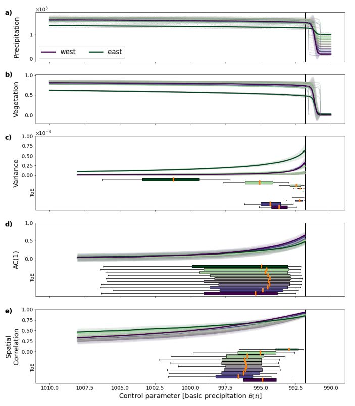
The conceptual model implements moisture-recycling from east to west in combination with decreasing moisture inflow from the Atlantic ocean. The latter one corresponds to a potential climate change scenario and acts as the forcing in the model. Once the point where the eastern cell tips to a low vegetation state is reached, the abrupt decline in vegetation reduces the inflow of recycled moisture in all the cells further to the west, thus inducing a tipping cascade. It is important to note that within one realization, all cells tip simultaneously, so the spread in the actual tipping point in Fig. 4b is a result of stochastic differences between the realizations. Before the Tipping Point, the resulting decline in precipitation is almost linear for all of the cells, compare the zoom-in into precipitation in Fig. S2. Interestingly, deforestation in the east-most cell mimicked by a artificial linear reduction of this cell’s vegetation state also induces a cascade of precipitation and vegetation tipping (see Fig. S3).
In Fig. 4, the vertical black lines mark the time when the total precipitation of at least one cell in at least one realization drops below the critical value for the first time. Thus, only time steps before entering this region are used in the resilience analysis. For all cells, variance, AC1 and spatial correlation as indicators of CSD are calculated on sliding windows and their change is assessed as the linear trends. For all indicators and all cells, the three indicators increase on average with almost no negative trends (see Fig. S4).
As defined in the Methods Section, the time of emergence (ToE) is the time when the trend of an indicator becomes significant for the first time. In Fig. 4 the median ToE is highlighted by an orange line and differs both between different cells and between different indicators for the same cell. For the eastern cell, variance is the first indicator to become significant. This early emergence is because this cell is the closest to a standalone tipping point, and so its variance is increasing towards infinity and thus the increase becomes significant earlier in time. This earlier increase shows that the tipping of the eastern cell triggers the cascading tipping of the other cells. Note that for this cell, the spatial correlation does not become significant in all realizations. For the second easternmost cell, the median ToE is comparable between the spatial correlation and the variance. For all other cells except the westernmost the spatial correlation outperforms the other indicators as an EWS (for the westernmost cell the AC1 has the earliest ToE). The comparison to the variance is especially striking, as the variance trend’s significance

emerges very late or not at all for these cells. One can thus conclude that the AC1 and spatial correlation become significant earlier and more often for the coupled cells, with spatial correlation being ahead in time for most cells. On the other hand, variance exhibits early significant trends for the (almost) uncoupled cells. Furthermore, an indicator is regarded more reliable when its trend consistently becomes significant at one time. This can be translated to a smaller spread in its ToE. It is apparent that the spread in ToE is smaller for spatial correlation for the highly coupled cells, indicating its robustness in systems with strong coupling. However, any indicator can sometimes have spuriously significant trends that lose their significance at a later time, so it is informative to also define a ‘permanent’ ToE. This ToE is defined as the time when the emergence of a significant trend is permanent for the rest of the time period, and is shown in Fig. S5. While this definition reduces the large uncertainty in the ToE of AC1, the choice of the method does not alter relations between the median ToEs of the different indicators. The overall result also stays the same: the spatial correlation is the most reliable and earliest indicator to have significant positive trends in coupled cells.
We conclude that, whilst their significance might emerge at different times, all three indicators are expected to increase for spatially extended systems like the ARF when approaching a critical transition. Moreover, the comparatively early and tightly spread time of emergence of the spatial correlation proves its reliability as an indicator of CSD in coupled systems. Consequently, if the ARF is losing resilience we would expect coherent and significant increases in all three indicators in observations of Amazon vegetation, with most pronounced signs in the spatial correlation.
Vegetation resilience in the Amazon basin
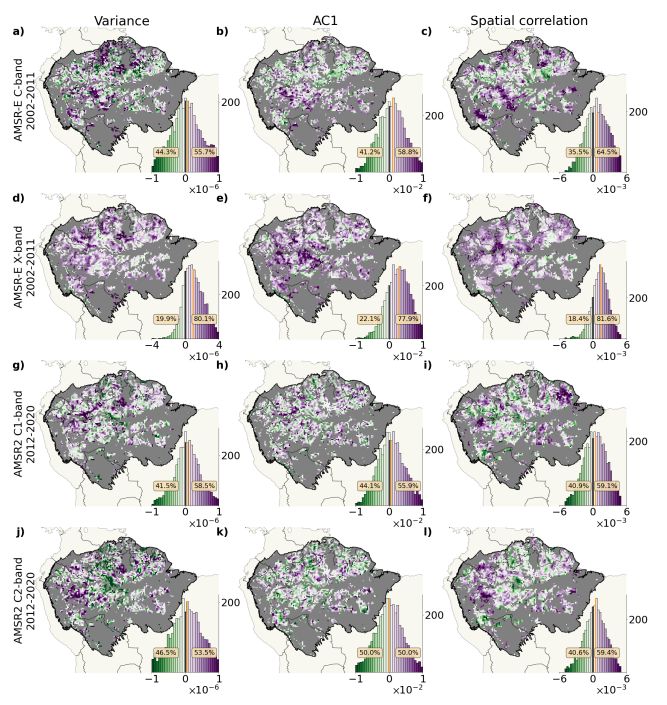
As the ARF is a spatially coupled system, similar to the simple moisture recycling model presented above, we expect to see increasing indicators of CSD in case of resilience loss. Three indicators are considered here, namely variance, AC1, and spatial correlation. The change in an indicator’s time series is quantified by the linear trend (see Methods section). Fig. 5 displays the spatial pattern of trends in the individual indicators as found for the different data sets. It is important to keep the different time spans of the two sensors in mind, as the results can only be compared within each sensor’s bands.
2002 - 2011 (AMSR-E): From July 2002 to September 2011, AMSR-E was active. The changes in the single indicators for AMSR-E’s C- and X-band are depicted in Fig. 5a)-f). For its C-band, the distributions of trends of all indicators have a positive median, so overall more cells exhibit a positive trend than not. Whilst the spatial distributions of trends in variance, AC1 and spatial correlation are distinct, in all three the positive trends cluster in the southwest and along the northern basin boundary. AMSR-E’s X-band has, for all three indicators, an even stronger tendency towards cells with a positive trend. The regions of positive trends comprise those of the C-band, but extend across the whole Amazon basin, with the only exceptions being some cells with non-positive trends in the east, close to the Amazon river.
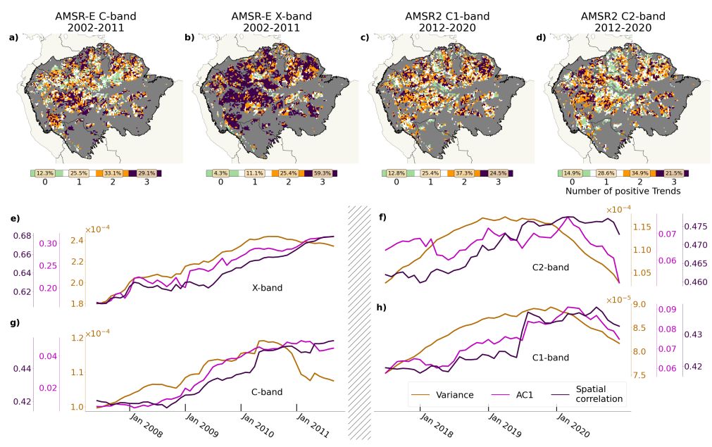
As explained above, in the case of CSD we would expect the changes in all three indicators to be coherent. Fig. 6 summarizes the results from the three indicators. The maps show the number of indicators exhibiting a positive trend at each grid cell. For AMSR-E’s C-band, Fig. 6a) confirms that the most prominent patch of positive trends in all indicators is the southwestern part of the Amazon basin. Further signs of extended resilience loss are noticeable along the northern basin boundary. For the X-band, the overall resilience loss of the ARF, yet especially pronounced in the southwest, becomes apparent in Fig. 6b and e). The time series of spatial averages suggest that the ARF as an interacting ecosystem has, on average, lost resilience over the years 2002 to 2011, with clear signals in both bands.
2012 - 2020 (AMSR2): Turning to the time period from August 2012 until December 2020, for which VOD data based on AMSR2 was analyzed, the signal is less clear (Fig. 5). Even so, except for the AC1 of the C2-band, the trends of all indicators are more often positive than negative. As for AMSR-E, the two bands in AMSR2 have different spatial trend distributions. For the C1-band, patches of positive trends, mostly in the variance and spatial correlation, are visible in the northeast as well as in the west. For the C2-band, the signals are stronger in the west but less pronounced in the northeast, and again strongest in the variance and spatial correlation. The spatial comparison of the trends in the three indicators in Fig. 6c) reveals that, based on the C1-band, the vegetation in the northeast of the Amazon basin has lost resilience. Even though no clear signals in this region were found for the years 2002-2011 based on AMSR-E’s


C-band, its X-band does show destabilization in this region already in the years before 2012. Considering the C2-band, positive trends co-occur mainly in the very west, where both bands from AMSR-E indicate a loss of resilience for the years before. The spatially averaged indicator time series clearly increase over the period until around mid-2019. Interestingly, from then on until the end of the study period, all time series decrease, although the decrease in the spatial correlation is marginal compared to the previous increases. We restrict our study period to years before 2020 as the data for excluding human land use is not available thereafter, but using a less conservative analysis we find that the indicators continue to decrease in the 2020- 22 period. Yet, this decrease could be explained by forest loss and the results for AMSR2 analyzed until 2022 cannot be relied on (see Fig. S6). Furthermore, AMSR2 also provides an Xband (10.7 GHz), for which results are shown in the supplement (Figs. S7 and S8) as the theory implies that it is less suitable for biomass assessment in the Amazon than the C-bands.
All results are robust with respect to the parametrization of the de-trending method STL (see Figs. S9 and S10), the size of the sliding windows (see Figs. S11 and S12), the measure of increase in the indicator time series (see Figs. S13 and S14), and the maximum distance that defines ‘neighbors’ (see Fig. S15).


