Soft Robots and Smart Movement

Table of Links

Abstract and 1 Introduction

2 Related Works

2.1 Pneumatic Actuation

2.2 Pneumatic Arms

2.3 Control of Soft Robots

3 PAUL: Design and Manufacturing

3.1 Robot Design

3.2 Material Selection

3.3 Manufacturing

3.4 Actuation Bank

4 Data Acquisition and Open-Loop Control

4.1 Hardware Setup

4.2 Vision Capture System

4.3 Dataset Generation: Table-Based Models

4.4 Open-Loop Control

5 Results

5.1 Final PAUL version

5.2 Workspace Analysis

5.3 Performance of the Table-Based Models

5.4 Bending Experiments

5.5 Weight Carrying Experiments

6 Conclusions

Funding Information

A. Conducted Experiments and References

5.3 Performance of the Table-Based Models

The size of the table to achieve acceptable kinematic modelling was set experimentally, as no previous references were available and previous works in the literature were very variable in terms of the number of data required. Furthermore, the possibility of an error occurring in the pneumatic system or the buffer of the vision acquisition system collapsing, together with the always present possibility of a leak in the segments, made it advisable to take data in small sessions and subsequently union of all of them. Since the data collection process was automated, this did not pose much of a problem.

Although the possibility that the ambient temperature was a factor that influenced the kinematics of the robot was considered during the dataset collection process, it was finally proven that small variations in temperature did not affect the behaviour.

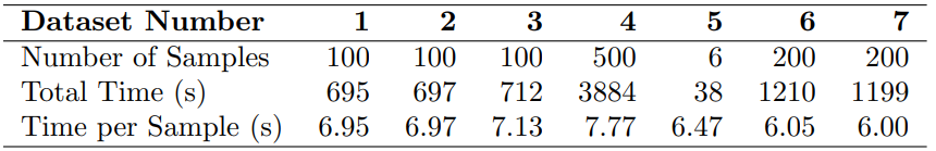
Table 3 shows the datasets that were taken, the total time necessary to obtain them and the average time per point. It should be taken into account that not all captured positions were finally used, since, if the camera did not correctly detect the positions of the three beacon spheres, it could not calculate the orientation of the trihedral and therefore returned an error code. Of the 1200 samples collected, 5% had to be discarded, leaving 1146 finally usable. The average time per point, considering all the datasets collected, was 6.76 s, with a standard deviation of 0.63 s. The low variability between capture processes proves the effectiveness of the automated method designed.

Once all the datasets were combined, the direct and inverse kinematic models presented here were validated. The validation of the direct model consisted of sending the robot a combination of inflation times and measuring the distance between the position reached, captured by the cameras, and that predicted by the table. Repeating the experiment for 40 points, the histogram of results presented in Figure 15 was observed. The average error is 4.27 mm, the median error 2.72 mm, and the standard deviation 1.99 mm.

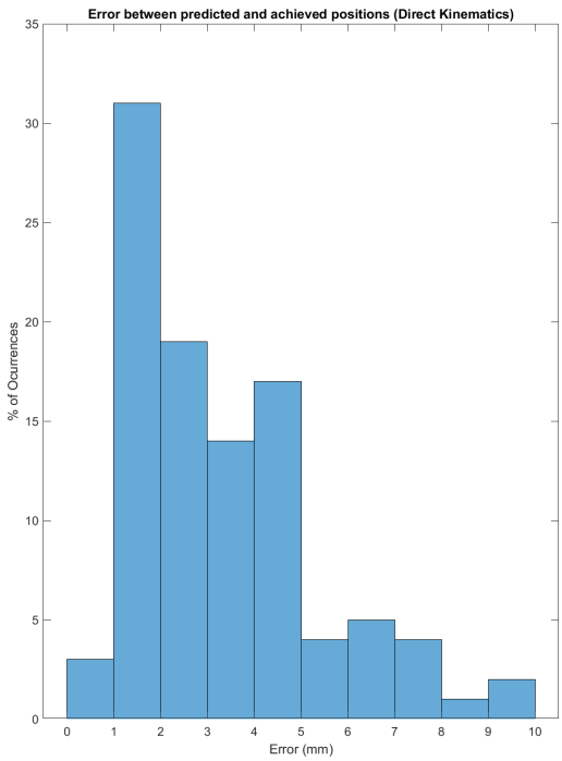
The high standard deviation and the shape of the histogram, tilted towards low values and with a very long tail, seem to indicate the existence of points where the model presents notable failures along with others with very good results. A future line of interest could be the detailed analysis of the workspace to locate where those regions of lower precision of the model are located and try to look for failures, perhaps leading to a greater density of points in the dataset.

In the same way, the inverse kinematic model was tested. To do this, PAUL was given a reference position and orientation to achieve, the necessary times were calculated, using the procedures referred to in Equations (16), and (17) inflation was carried out. Subsequently, the position captured with the cameras was compared with the desired one.

As expected, the existence of redundancies, in which equal position values are achieved with very different combinations of inflation times, introduces large uncertainties in the model, which the triangulation presented is not able to capture.

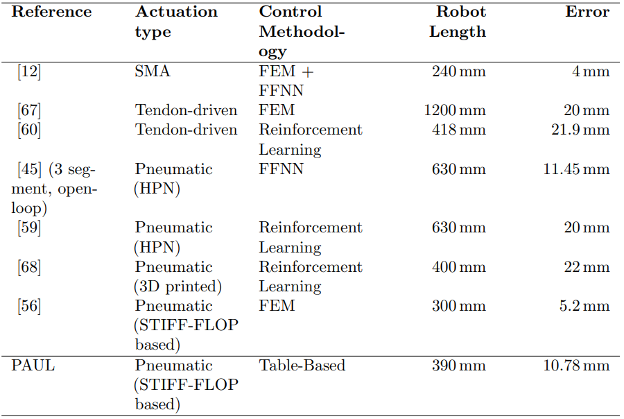
Specifically, the inverse kinematic model has an average error of 10.78 mm, a median error of 9.22 mm and a standard deviation of 5.98 mm. While these errors may seem high, they are compared in Table 4 with other open-loop controllers presented in the literature. It can be clearly seen that they are in line with the results obtained and that they are even better than those obtained by smaller robots, where one would expect, due to the smaller working space, a higher accuracy (at least in data-driven models).

It is worth highlighting, however, two experiments in which PAUL performed very satisfactorily, because the area of operation was restricted to a region where no redundancies were found to exist. They are available in the video of Appendix A.

In the first of them, the robot was forced to reach a set of points located on the horizontal basis plane, also forcing the lower end of the last segment to be parallel to said

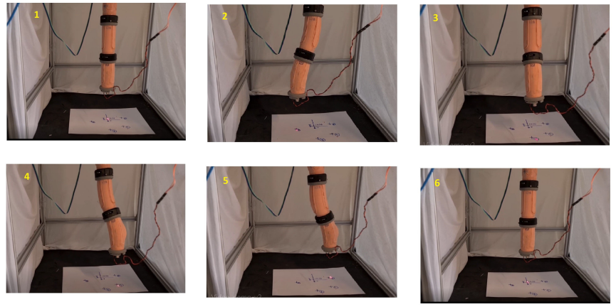
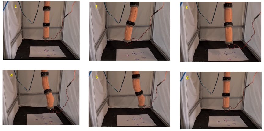
plane. In all of them, errors less than 7 mm were achieved. Figure 16 shows the results of said experiment. With the aim of facilitating the understanding of the experiment, the beacon was changed for a laser pointer that points to the desired points, on which targets with a radius of 5 mm have been marked, allowing the accuracy achieved to be checked.

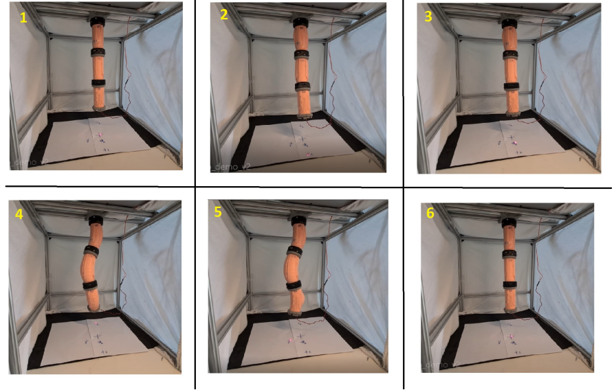
In the second experiment, shown in Figure 17, points on the lower horizontal plane were also taken as reference, but without imposing that the lower face of the robot should remain parallel to it. In this case, accuracies of 2 cm were achieved.

Although the inverse kinematic model therefore presents acceptable results, it must be commented that, in all these experiments, due to the geometry and material of the robot, at the moment in which PAUL reaches the desired position, it tends to acquire a movement damped oscillation. An attempt has been made to reduce it, despite everything, it is a very intrinsic phenomenon to the robot that is difficult to solve. A future line proposed, in this sense, is to try to rigidify the robot by introducing negative pressures that generate vacuum.