This paper is available on arxiv under CC 4.0 license.
Authors:
(1) Eleonora Alei, ETH Zurich, Institute for Particle Physics & Astrophysics & National Center of Competence in Research PlanetS;
(2) Björn S. Konrad, ETH Zurich, Institute for Particle Physics & Astrophysics & National Center of Competence in Research PlanetS;
(3) Daniel Angerhausen, ETH Zurich, Institute for Particle Physics & Astrophysics, National Center of Competence in Research PlanetS & Blue Marble Space Institute of Science;
(4) John Lee Grenfell, Department of Extrasolar Planets and Atmospheres (EPA), Institute for Planetary Research (PF), German Aerospace Centre (DLR)
(5) Paul Mollière, Max-Planck-Institut für Astronomie;
(6) Sascha P. Quanz, ETH Zurich, Institute for Particle Physics & Astrophysics & National Center of Competence in Research PlanetS;
(7) Sarah Rugheimer, Department of Physics, University of Oxford;
(8) Fabian Wunderlich, Department of Extrasolar Planets and Atmospheres (EPA), Institute for Planetary Research (PF), German Aerospace Centre (DLR);
(9) LIFE collaboration, www.life-space-mission.com.
Table of Links
Appendix A: Scattering of terrestrial exoplanets
Appendix C: Bayes’ factor analysis: other epochs
Appendix D: Cloudy scenarios: additional figures
3. Results
In this section we show the results from the retrievals on the grid of different input spectra (see Table 1) assuming the baseline parameters listed in Table 2. We start by analyzing the retrieved spectra (Section 3.1) to offer a broad overview of the retrieval performance.
Then, we study the retrieved P-T profiles (Section 3.2), the planetary parameters (Section 3.3) and abundances (Section 3.4). We also ran additional retrievals of the same scenarios (shown in Table 1) by varying R and S/N. We compare the results of these retrievals in Section 3.5.
3.1. Retrieved emission spectra
The main output of the Bayesian retrieval framework are the posterior distributions of the parameters, necessary to produce the oretical spectra, that best match the data. The posteriors can be visualized as an N-dimensional space that is a subset of the larger N-dimensional prior space, N being the number of parameters.
Each point included in the posterior space has N coordinates and represents a combination of N parameters that, if fed to the theoretical spectral model, would produce a spectrum that was determined by the Bayesian framework to resemble the observed spectrum.
Table 3: Summary of the parameters used in the retrievals, their expected values and their prior distributions.
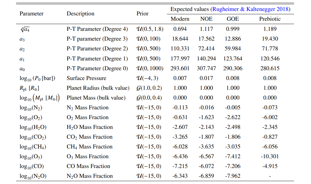
Table 4: References for the molecular opacities used in the retrievals.

Table 5: References for the CIA and Rayleigh opacities used in the retrievals.

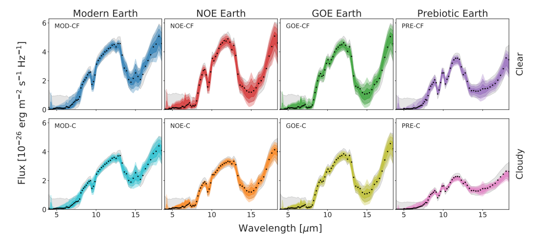
From the available sets of parameters within the posteriors that the routine has calculated, we can therefore produce "retrieved spectra". These are shown in Figure 1. Each subplot presents the results for a specific model.
The input spectrum is binned down to R = 50. Every flux point is represented by black dots and the uncertainty determined by LIFEsim is shown as a gray shaded area. The retrieved spectra are color-coded according to Table 1.
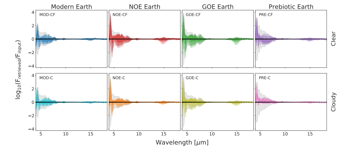
The color of the shading is scaled according to the uncertainty in the retrieved spectra: the 1-σ uncertainty region is shown in a darker color than the 2- and 3-σ regions. Similarly, Figure 2 shows the logarithm of the ratio between the retrieved emission spectrum and the input emission spectrum for each scenario.
The retrieved spectra are generally in good agreement with the input spectra (within 1 σ) for all considered cases. This shows that our retrieval framework is able to reproduce the simulated input spectra, regardless of the complexity of the input model (in terms of thermal and abundance profiles, and cloud coverage). However, we notice regions with larger uncertainties, especially at wavelengths shorter than ≈ 8 µm.
Here, the ratio between the retrieved spectra and the input spectrum (as shown in Figure 2) reaches up to a few orders of magnitude. Such differences are, however, still within the noise uncertainty (gray shaded areas). Smaller differences can be noticed in the main CO2 band at ≈ 15 µm.
Since the noise is not as high as it is in the short wavelength range, these differences are probably due to discrepancies in the opacity tables (see Section 4.4).
The parameter estimation routine included in the Bayesian retrieval framework has the task of minimizing the difference between model output and data. For this, no detailed parameterization of the relevant physical processes are required. Many of the relevant physical and chemical parameters are correlated (e.g. the planetary mass and the pressure, the pressure and the chemical abundances), often in a non linear way.
It is therefore possible for the parameter estimation routine to produce similar spectra as the full (physical) input model over a diverse set of parameters, as a result of such correlations. It is appropriate therefore to question whether the parameter estimation routine results are on the one hand physically representative, or whether degeneracies and systematics between the retrieved parameters could be influencing the results. The next sections will explore these issues in more detail.
3.2. Retrieved P-T profiles
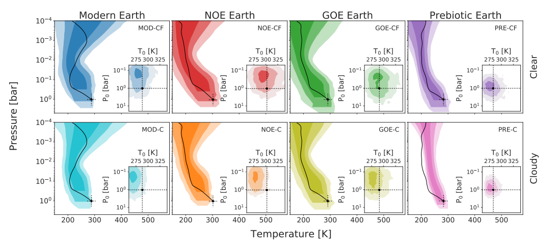
In Figure 3 we show the retrieved P-T profiles compared to the input profiles for all combinations of the four epochs (columns) and the two cloud coverages (rows).
The vertical shape of the retrieved P-T profiles in the lower atmosphere (pressures ≥ 10−2 bar) roughly follows that of the true P-T profiles. In most cases the true profiles are contained within the 1-σ uncertainty envelope. As in Paper III, the uncertainties grow larger at higher altitudes (pressures ≤ 10−2 bar).
This indicates that, for the quality of the input spectra we consider for this study, it is not possible to distinguish atmospheres with a stratospheric temperature inversion (i.e. the Modern Earth scenario) from those with an isothermal stratosphere (i.e. the NOE, GOE, and Prebiotic scenarios). This retrieval limitation is a result of the small overall contribution of the upper atmospheric layers to the planet’s MIR emission spectrum.
A few additional inconsistencies between the retrieved and input P-T profiles are also apparent in the lower altitudes (high pressures). A general feature in the three biotic epochs (Modern, NOE, and GOE Earth) is the retrieval of underestimated values for the ground pressure P0 (∼0.1 bar as opposed to the true value of ∼1 bar).
This occurs for both the cloud-free and cloudy spectra. Such offset could be explained by systematic differences between the radiative transfer models used to produce and to retrieve the simulated spectra. We will discuss this in more detail in Section 4.4.
The ground temperatures T0 are on average well retrieved for all clear sky scenarios. In contrast, the retrievals performed for the cloudy spectra systematically underestimate T0, with differences between the retrieved and true value . 25 K. These results have an impact on assessing the habitability of the simulated exoplanets, which will be discussed in more detail in Section 4.
For the Prebiotic Earth input spectra, the retrievals provide estimates for P0 and T0 that are in agreement with the true parameter values. Furthermore, the overall uncertainties on the retrieved P-T profile are generally smaller than for the other epochs.
However, for the cloudy Prebiotic Earth (PRE-C) spectrum, the retrieved P-T profile is a few tens of Kelvin warmer than the true value in the intermediate layers of the atmosphere (∼ 10−1 to ∼ 10−3 bar).
This effect is likely related to the much weaker emission features in the cloudy Prebiotic Earth scenario compared to the other epochs. We will discuss the impact of neglecting clouds in the retrievals in Section 4.2.
3.3. Retrieved planetary parameters
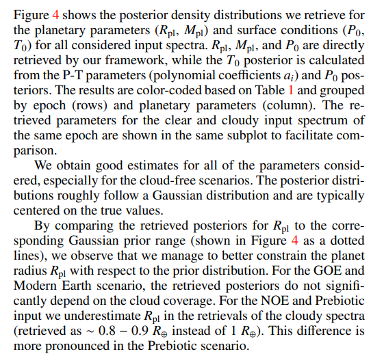
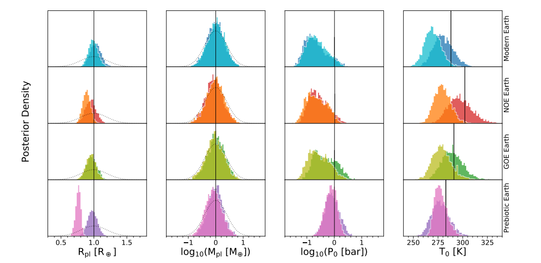
underestimate the surface temperature. The standard deviation of the retrieved T0 posteriors is roughly ±20 K for all biotic scenarios.
This is in agreement with the findings made in Paper III. The spread of retrieved posteriors could potentially be reduced by increasing the R or S/N of the input spectra (see Section 3.5). Observing strategies for the trade-off between R and S/N will be addressed in Section 4.3.
3.4. Retrieved chemical abundance parameters
Figure 5 shows the retrieved posterior distributions for the main atmospheric gases. We again arrange the various scenarios by epoch (row), and atmospheric species (column) and use the color-coding from Table 1.
The results for the clear and the cloudy retrievals of one epoch are shown in the same subplot to facilitate comparison.
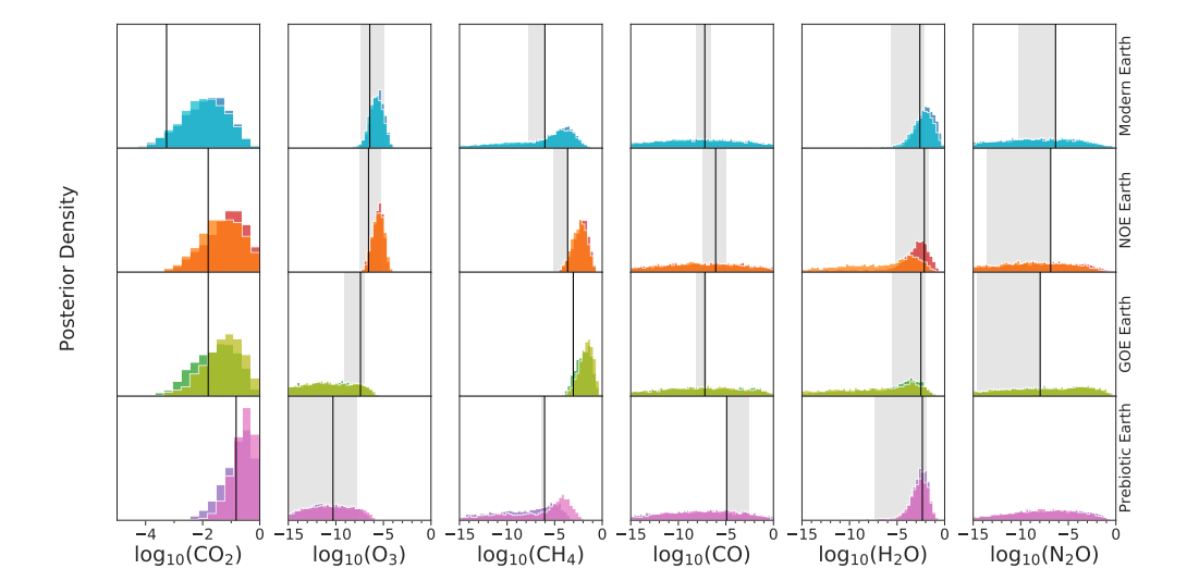
We plot our expected abundances (listed in Table 3), which are the weighted means (with respect to the pressure) of the original abundance profiles, as black vertical lines. If no true value is plotted, the molecule is not present in the input spectrum. We further indicate the range of variability of the true, pressuredependant abundance profiles (minimum to maximum) via the shaded gray area in each subplot.
We adopt the same posterior classification scheme that was introduced in Paper III, for an easier comparison of the results. This scheme divides the retrieved posteriors into the following four classes:
– Constrained (C): The posterior is best described by a Gaussian distribution. This implies that abundances both significantly lower and higher than the true value can be ruled out.
– Sensitivity limit (SL): The abundance is at the retrieval’s detection limit for the species. The posterior exhibits a distinct peak. However, low abundances are not ruled out. The posterior is best described by the convolution of a soft-step function with a Gaussian.
– Upper Limit (UL): The posterior resembles a soft-step function. Large abundances can be excluded, low ones cannot.
– Unconstrained (UC): We cannot retrieve information on the atmospheric abundance. The posterior resembles a constant function over the full prior range.
For further details on the specifics of the posterior classification we refer the reader to the Appendix B of Paper III.
We obtain UC posteriors for the abundances of N2 and O2 in all retrievals performed. In accordance with the findings presented in Paper III, these molecules are not detectable in any of the considered scenarios. This finding indicates that the corresponding CIA spectral signatures are too weak to be detectable in the considered input spectra with R = 50 and S/N = 10.
To increase readability, we choose not shown the retrieval results for N2 and O2 in Figure 5. The posterior distributions of these molecules can however be found in the corner plots in Appendix B. Similarly, the trace gases N2O and CO were not detected in any of our retrievals, obtaining unconstrained posteriors for all epochs.
The MIR absorption features of these molecules at the considered abundances are also too weak in the considered input spectra to be constrained in our retrievals. This can be seen by the flat posterior distributions for both species in all considered cases (see Figure 5).
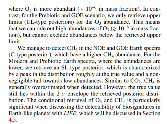
We detect CO2 in all retrievals and the received posterior distributions are generally Gaussian-like (C-type posteriors). Our results suggest that the median abundances of the different posterior distributions are higher than the true value for all the epochs.
However, in the Prebiotic, GOE, and NOE scenarios the true abundances still lie within the 1-σ envelope of the retrieved abundances. For the Modern Earth scenarios, the true value lies within the 3-σ range of the retrieved posterior. This is consistent with a "compensation effect" whereby the retrieval framework is correcting for the underestimated pressure.
The degeneracy between chemical composition and atmospheric pressure is well known and it was already encountered in Paper III (see Section 4.1). All retrieved CO2 posteriors span about 3 orders of magnitude (3 dex). They all appear very similar even though the expected values of CO2 span from roughly 0.01% (Modern Earth) to the order of 10% (Prebiotic Earth).
This forbids the use of CO2, one of the major absorbers in the atmosphere, as discriminator between the considered epochs. To reduce the variance in the retrieved abundances, an increase in R and/or S/N might be recommended (see Section 3.5).
For the remaining species (O3, CH4, and H2O) the retrieval results depend on the considered epoch:
O3 is retrieved accurately in both the Modern Earth and NOE Earth scenarios (C-type posteriors). These are the two cases
3.5. Runs at higher resolution and/or signal-to-noise ratio
In this Section, we investigate whether our retrieval results can be improved by increasing the quality (R and/or S/N) and thus the information content of the input spectra. We ran ancillary retrievals for the 8 scenarios and choose the following combinations of R and S/N [5] :
– R = 50 and S/N = 10 (the reference case);
– R = 100 and S/N = 10;
– R = 50 and S/N = 20;
– R = 100 and S/N = 20;
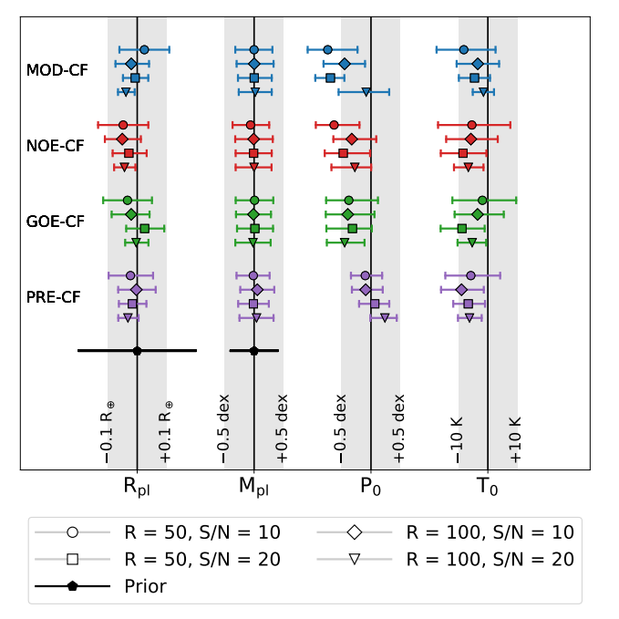
We provide a summary of the results obtained from these additional retrieval runs in Figures 6 (planetary parameters) and 7 (abundances). Results from the different ancillary runs are represented using different markers.
The results for the different epochs are color-coded according to Table 1. Here, we only show the results for the clear input spectra. The plots corresponding to the cloudy scenarios can be found in Appendix D.
We are particularly interested in significant increases in accuracy (i.e. the retrieved values agree better with the input "truth") or in precision (i.e. the posterior’s variance is reduced). For higher S/N we expect more precise results, since the uncertainty in the input spectrum is lower. This yields stronger constraints on the model parameters.
An increase in R should allow for a more robust identification and characterization of the spectral features and thus more accurate retrieval results. Both increased accuracy and/or precision could allow us to differentiate between the different epochs (and generally between different planets) more clearly. This will be of great importance, especially when searching for signatures of life in exoplanetary atmospheres (see Section 4.5).
We should point out that in our current simulation setup, which ignores (systematic) instrumental noise terms, doubling R at a constant S/N means doubling the integration time, while doubling S/N at a constant R means, roughly, quadrupling it6 . This information is crucial for the mission planning and will be further discussed in Section 4.3.
In Figure 6, we notice that increasing the S/N to 20 while keeping R = 50 (square markers) generally results in a narrower posterior for Rpl. We observe a reduction in variance of the Rpl posterior by up to a factor of 2 compared to the reference case (R = 50, S/N = 10; the circular markers). An increase in R (R = 100, S/N = 10; the diamond markers) causes the variance of the Rpl posterior to shrink to about 70% of the reference case variance.
In contrast, we observe no noticeable gain in the accuracy of the retrieved value for Rpl when increasing S/N and R at the same time. On the other hand, the precision of the measurement at R = 100, S/N = 20 improves significantly, with the variance of the Rpl posterior shrinking up to three times compared to the reference case.
We further find that the retrieval of the planetary mass Mpl does not improve significantly when moving to higher R and S/N input spectra. We observe no significant increase in both accuracy and precision. This finding is consistent with the results shown in Paper III.
The underlying reason for this observation is the degeneracy between the surface gravity (and thus also Mpl) and the abundances of trace gases (see e.g. Paper III, Mollière et al. 2015; Feng et al. 2018; Madhusudhan 2018; Quanz et al. 2021).
Since gravity and abundances are involved in the hydrostatic equilibrium, it is possible to reproduce the same spectral feature using different combinations of these parameters. This broadens the variance of the posteriors of Mpl and of the atmospheric species.
Increasing the quality of the input spectrum does improve the accuracy of the retrieval for P0 in the clear Modern Earth (MODCF) case. The results for the other epochs do not exhibit a similar trend with increasing input quality.
This failure to retrieve accurate ground pressure estimates is likely rooted in differences between the opacity tables used by the retrieval framework and the ones used to calculate the input spectra (see Section 4.4 for more details).
Additionally, no noticeable decrease in the variance of the retrieved P0 estimate is present for higher values of R or S/N. This is likely a result of the pressure-abundance degeneracy, which has already been described in Section 3.4.
For the surface temperature T0, we do not notice any substantial improvements in the accuracy of the retrieved values when increasing R or S/N. However, as for Rpl, we observe a significant reduction in the variance of the posteriors when increasing S/N and R.
Compared to the reference case, the uncertainty in T0 is reduced by a factor of 2 for the runs with S/N = 20 and to about 70% of the reference variance for the runs with R = 100. These improvements in temperature accuracy could be crucial when assessing the potential habitability of an observed exoplanet.
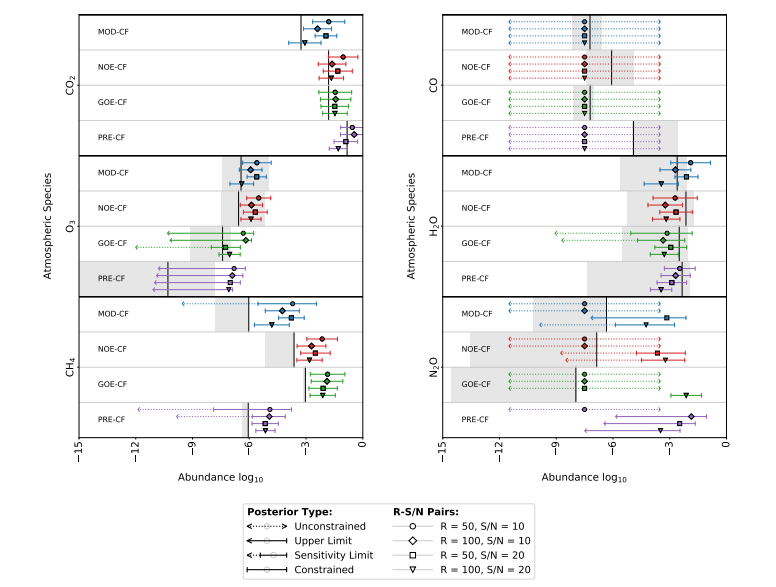
In Figure 7 we summarize the retrieved posterior distributions in the abundances for the reference case (R = 50 and S/N = 10, circular markers) and all other R and S/N combinations. The abundance posteriors are classified according to our classification scheme (see Section 3.4 and Paper III).
Generally, we observe that increases in both S/N and R do not significantly improve the accuracy nor the precision of the retrieved posteriors for the majority of the scenarios. This is again the result of the pressure- and gravity-abundance degeneracies.
In particular, the pressure-abundance degeneracy is responsible for the shifts with respect to the true values, whereas the gravityabundance degeneracy defines the variance of the abundance posteriors.
The effects of the pressure-abundance degeneracy can be noticed for CO2 in the clear Modern Earth (MOD-CF) scenario. For the reference case (circular marker) we strongly underestimated P0, which is compensated by an overestimation in the CO2 abundance.
As we move to higher R and S/N input spectra, our estimate for P0 improves, which results in better accuracies for the retrieved CO2 abundance. The same connection between P0 and the retrieved abundances can be seen for all other constrained species.
In contrast, the variance of the CO2 posterior does not decrease significantly with increases in R and S/N since it is limited by the variance of the Mpl posterior (due to the gravityabundance degeneracy), which is the same for all considered cases. While this behaviour describes the results for most species well, there are some noteworthy exceptions that we will discuss here.
Firstly, there could be a tentative detection of O3 (an SL posterior) in the clear GOE Earth (GOE-CF) epoch when increasing the S/N to 20 (square marker). If also the resolution is increased to R = 100 (triangular marker), we could better constrain the O3 abundance. Purely increasing R to 100 would not improve the accuracy or the precision of O3 (diamond marker).
Similarly, increasing the S/N would allow for a detection of CH4 in all four epochs, which was not possible for the reference case (circular marker). However, the retrieved CH4 abundances are one to two orders of magnitude higher than the truths.
Results suggest similar, but less pronounced systematic offsets with respect to the true values for the other constrained species. These offsets are likely the result of a combination of the degeneracy between P0 and the abundances and systematic errors, such as differences in the molecular line lists (see Section 4.4).
Both O3 and CH4 are of particular interest for astrobiology, since they are indicative of disequilibrium chemistry in the atmosphere and could indicate the presence of biological activity on the planet. We will discuss this in more detail in Sections 4.3 and 4.5.
Furthermore, an increase in S/N would enable a robust detection of H2O in the clear GOE Earth (GOE-CF) epoch (C- instead of SL-type posterior). On the contrary, increasing the resolution alone does not have the same effect.
Finally, CO is unconstrained for all epochs and R-S/N pairs, which indicates that this species could not be detected in an Earth-like atmosphere with LIFE. Similarly, none of the runs were able to fully constrain the N2O abundance.
The retrieval can only provide upper limits on the N2O abundance, which often only manage to rule out atmospheric abundances greater than 1% in mass fraction. The retrieval is therefore not sensitive to these molecules – their spectral signatures are too small compared to the LIFEsim noise to be detected even in the best considered scenario.
An exception would be the clear GOE Earth at R = 100 and S/N = 20 scenario, for which we retrieve a wrong estimate of N2O (around 1% in mass fraction), about 6 orders of magnitude larger than the true value. The retrieval is most likely fitting the noise and/or spectral signatures of most of the other species at shorter wavelengths (λ . 8 µm).
Hence, when analyzing observations of potentially habitable terrestrial planets, we should be mindful not only of the false positive mechanisms that may be active in the atmosphere, but also of the false positives that the retrieval routines can infer.
One could try to solve this issue by averaging over multiple retrieval runs, or by reducing the prior space with inferred knowledge from independent observations.
The retrievals of the ancillary cloudy input spectra (shown in Appendix D) do not show any noticeable improvement in either accuracy or precision for all scenarios with increased R and S/N. The values of Rpl and T0 are still underestimated for all the scenarios.
However, all considered R and S/N combinations still allow for an atmospheric abundance characterization for the cloudy input spectra. This analysis is subject to similar limitations as those already discussed for the subset of clear input spectra. The impact of clouds in retrievals will be discussed in more detail in Section 4.2.
[5] We remind the reader that the S/N refers to the value at a reference wavelength of 11.2 µm.
[6] We refer the reader to the Appendix of Paper I, where we show a breakdown of the typical noise contributions for planets detected around Solar-type stars.
This paper is available on arxiv under CC 4.0 license.

