This paper is available on arxiv under CC 4.0 license.
Authors:
(1) Eleonora Alei, ETH Zurich, Institute for Particle Physics & Astrophysics & National Center of Competence in Research PlanetS;
(2) Björn S. Konrad, ETH Zurich, Institute for Particle Physics & Astrophysics & National Center of Competence in Research PlanetS;
(3) Daniel Angerhausen, ETH Zurich, Institute for Particle Physics & Astrophysics, National Center of Competence in Research PlanetS & Blue Marble Space Institute of Science;
(4) John Lee Grenfell, Department of Extrasolar Planets and Atmospheres (EPA), Institute for Planetary Research (PF), German Aerospace Centre (DLR)
(5) Paul Mollière, Max-Planck-Institut für Astronomie;
(6) Sascha P. Quanz, ETH Zurich, Institute for Particle Physics & Astrophysics & National Center of Competence in Research PlanetS;
(7) Sarah Rugheimer, Department of Physics, University of Oxford;
(8) Fabian Wunderlich, Department of Extrasolar Planets and Atmospheres (EPA), Institute for Planetary Research (PF), German Aerospace Centre (DLR);
(9) LIFE collaboration, www.life-space-mission.com.
Table of Links
Appendix A: Scattering of terrestrial exoplanets
Appendix C: Bayes’ factor analysis: other epochs
Appendix D: Cloudy scenarios: additional figures
2. Methods
We start by discussing the details of the input spectra that were used in this study (Section 2.1). We then discuss the updates on the Bayesian retrieval routine (Section 2.2). We describe the assumptions that our model takes into account and the main potential source of systematic errors in the retrievals in Section 2.3.
2.1. Input spectra and scenarios
We consider spectra corresponding to four different evolutionary epochs of Earth: the prebiotic Earth (3.9 Ga), the Earth shortly after the Great Oxygenation Event (2.0 Ga), the Neoproterozoic Oxygenation Event (0.8 Ga), and Modern Earth. All considered Earth spectra were produced by Rugheimer & Kaltenegger (2018).
These self-consistent spectra were produced using a 1D convective-radiative transfer model loosely coupled with a 1D climate model and a 1D photochemistry model. The authors accounted for the thermal chemistry and the photochemistry of more than 55 species.
The atmospheres were modeled up to 10−4 bar and split into 100 layers. The radiative forcing of clouds is included by adjusting the surface albedo of the planet.
The results of the photochemistry-climate-radiative model were then fed to a line-by-line radiative transfer model to produce emission spectra. The line lists and the pressure broadening coefficients were from to the HITRAN 2016 database (Gordon et al. 2017).
Surface scattering was included in the calculations, assuming 70% ocean, 2% coast, and 28% land. In some scenarios, a partial cloud coverage was directly included in the calculation of the emission spectrum.
In these cloudy cases, the authors assumed a 60% cloud coverage (split into 40% water clouds at 1 km altitude, 40% water clouds at 6 km altitude, and 20% ice clouds at 12 km altitude) consistent with an averaged Earth cloud model. Aerosol was not included in the calculation.
The model has been validated from the visual to the mid-infrared wavelength ranges with observations of Earth (Kaltenegger et al. 2007; Kaltenegger & Traub 2009; Rugheimer et al. 2013). For further details, we refer the reader to Rugheimer & Kaltenegger (2018).
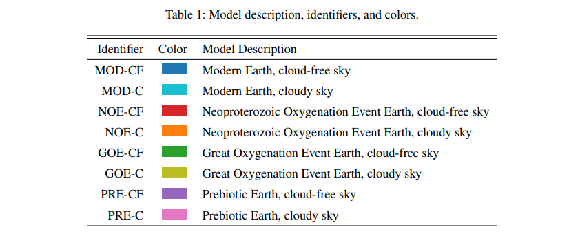
For each epoch, we consider both clear sky and cloudy sky spectra, which yields a total of 8 scenarios. We assigned every modeled scenario an identifier and a specific color, as listed in Table 1. We will use these identifiers throughout the remainder of the paper.
We simulate observations with LIFE via the LIFEsim tool (see Paper II for a description of the simulator). LIFEsim estimates the wavelength-dependent S/N considering all major astrophysical noise sources (stellar leakage, local zodiacal dust emission, and exo-zodiacal dust emission). We consider an Earth-sized planet on a 1 AU orbit around a Sun-like star at 10 pc distance.
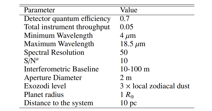
For our baseline analyses we assumed the nominal simulation parameters for LIFEsim as summarized in Table 2 (see Paper I and Paper II for details). We consider an exo-zodi level of 3 times the local zodiacal dust density, based on the results from the HOSTS survey (Ertel et al. 2020).
2.2. Updates on the Bayesian retrieval framework
We denote the input spectra from Section 2.1 as the "true spectra." To simulate a LIFE-like observation of these targets, we run LIFEsim on the true spectra, thus obtaining simulated "observed spectra."
We then perform a retrieval on the observed spectra using petitRADTRANS (Mollière et al. 2019) as "forward model" in the retrieval routine, and the Bayesian sampler model pyMultiNest (Buchner et al. 2014) as "parameter estimation routine" (cf. Paper III).
The theoretical 1D atmospheric model petitRADTRANS (Mollière et al. 2019) applies the radiative transfer equation to calculate spectra corresponding to a set of parameters. These parameters describe the bulk parameters (planetary mass and radius), the pressure-temperature (P-T) structure (approximated by a fourth-order polynomial), and the chemical composition of the atmosphere.
Our Bayesian retrieval framework recursively draws combinations of parameters from a set of "priors" that describe the "a priori" probability distribution of each parameter (listed in Table 3) and uses the forward model to compute the corresponding spectra.
Then, the Bayesian framework tests how well these calculated spectra fit the observed one using a "likelihood" function (see Eq. (3) in Paper III). In order to sample the prior space efficiently, our retrieval relies on the parameter estimation routine pyMultiNest (Buchner et al. 2014), which is based on MultiNest (Feroz et al. 2009).
This routine applies the Nested Sampling algorithm (Skilling 2006) to fit the theoretical spectral model to the observed spectrum, and thereby yields estimates and uncertainties for the model parameters.
These estimates are the "posterior probability distributions" (or "posteriors"). The posteriors contain the information on which combinations of model parameters best describe the observed spectrum. For more details about the Bayesian retrieval framework, we refer the reader to Paper III.
In our previous work, we argued that effects of scattering on simulated mid-infrared spectra are negligible at the considered resolutions and LIFEsim noise patterns. In that study, we had to be particularly mindful of the computing time.
The version of petitRADTRANS used in Paper III only allowed to calculate spectra at R = 1000, which were subsequently binned down to the resolution of the input spectrum (R = 35 − 100 in Paper III). Calculating a spectrum at R = 1000 excluding scattering required ≈ 0.5 seconds, whereas including scattering required ≈ 18 seconds.
Since millions of spectra have to be calculated for a single Bayesian retrieval, including scattering was prohibitive with respect to the computing time, especially when considering a large grid of retrieval runs.
Recent updates to petitRADTRANS have enabled us to compute spectra at any resolution, provided a grid of correlated-k tables at that resolution is available. These tables can be produced with petitRADTRANS by binning down the R = 1000 opacity tables.
We compiled a correlated-k opacity database for R = 50 and used it to produce spectra directly at this resolution. This reduces the computation time per spectrum significantly and allows us to compute emission spectra in ≈ 0.04 seconds when excluding scattering, and in ≈ 0.5 seconds when including scattering.
This reduction in computing time allows us to include scattering in the theoretical spectral model.
Other updates on petitRADTRANS were performed. The treatment of collision-induced absorption (CIA) was modified by updating the interpolation of the CIA tables, originally in FORTRAN, to Python. Minor variations in the interpolation options (log-linear compared to nearest neighbor in Paper III) make the new model not directly comparable with its previous version.
However, at Earth-like conditions, the differences in the CIA signature on the spectrum remain negligible. Also, the CIA features impact mostly the short wavelengths (λ < 6 µm), where the LIFEsim noise is large.
Furthermore, the treatment of scattering was updated. Originally implemented in petitRADTRANS only for gaseous planets (see Mollière et al. 2019), it was adapted to include the scattering by a rocky surface.
More information on the new implementation of scattering can be found in Appendix A, as well as the petitRADTRANS documentation[3] . This new version of petitRADTRANS is available in the main GitLab repository[4] .
Using the updated retrieval framework, we run retrievals for the eight different spectra introduced in Section 2.1. We retrieve the same parameters as in Paper III and leave most prior distributions unchanged. An exhaustive list of the parameters and priors used, and the corresponding expected values for the different epochs, are listed in Table 3.
Most priors are represented by a boxcar function (hereafter "uniform" priors): every value is equally probable if within a certain range. Two notable exceptions are the priors for the planetary radius Rpl and the logarithm of the planetary mass log10(Mpl), whose priors are Gaussian.
The prior we assumed on Rpl is based on the radius estimate expected from observing a terrestrial planet with LIFE during its search phase (see Paper II for details).
The log10(Mpl) prior was inferred from Rpl using the statistical mass-radius relation presented in Chen & Kipping (2016) (see Paper III for details).
2.3. Assumptions and discrepancies
When performing retrievals, we are limited by the maximum number of parameters retrieved in a reasonable computing time. For this reason, we need to make a few simplifications:
1. As in Paper III, we parameterize the P-T profile in the retrieval by a fourth order polynomial.

Table 2: Simulation parameters used in LIFEsim for the baseline analyses.

2. We assume the abundances of the considered species to be independent of altitude.
3. Our retrieval framework does not model clouds for any of the considered scenarios. This is a strong simplification for the cases where we retrieve cloudy input spectra.
However, this retrieval approach allows us to investigate the biases on the results obtained when retrieving a cloudy spectrum assuming a cloud-free atmosphere.
The addition of a cloud model to our retrieval framework will be tackled in a future study
4. A surface reflectance of 0.1 is assumed for all the wavelength range. This is a common value for water-rich habitable terrestrial planets, dominated by the low IR reflectance of oceans and ice.
In contrast, Rugheimer & Kaltenegger (2018) used P-T profiles that were self-consistently calculated by their climatephotochemistry model to generate the input spectra.
The chemical abundance profiles were also altitude-dependent and calculated self-consistently by the climate-photochemistry model.
In order to compare the results of the retrievals with the input, we approximate the input P-T and abundance profiles to calculate expected values of the parameters considered in the retrievals.
Regarding the thermal structure of the atmosphere, we determine the expected values of the polynomial coefficients (a4, a3, a2, a1, a0) listed in Table 3 by fitting a fourth-order polynomial to the self-consistent P-T profiles. As for the abundances, we assume the weighted means over the pressure grid of the altitude-dependent abundance profiles.
This is sensible, since the denser layers of the atmosphere (which corresponds to higher pressures) are generally the ones that contribute more to the spectrum. The expected values for the considered species are listed in Table 3 as well.
For what concerns the surface reflectance, Rugheimer & Kaltenegger (2018) considered a wavelength-dependent reflectance. However, the reflectance still averaged to 0.1 in the wavelength range of interest. We would therefore not expect large variations due to this parameter.
There are also differences between the opacity tables that the two models use. We used the default set of opacities for petitRADTRANS as presented in Mollière et al. (2019). We added the N2O opacity from the ExoMol database (Chubb et al. 2021). The CIA opacities are taken from the HITRAN database.
Details and reference papers corresponding to the opacity linelists are shown in Tables 4 and 5. In contrast, the input spectra were calculated using HITRAN 2016 opacities (Rugheimer & Kaltenegger 2018).
Differences in line-lists and broadening coefficients are therefore to be expected and may cause biases in the results.
Due to these differences in the atmospheric models, we would imagine to find some small discrepancies between the spectra that were published in Rugheimer & Kaltenegger (2018) and the ones that our framework can calculate. We will discuss this particular aspect in Section 4.4.
[3] https://petitradtrans.readthedocs.io
[4] https://gitlab.com/mauricemolli/petitRADTRANS
This paper is available on

